Stereographic projection#
In this tutorial, we will plot vectors in the stereographic projection.
The stereographic projection maps a sphere onto a plane and preserves angles at which curves meet. In orix, the projection is used to project unit Vector3d objects onto the equatorial plane represented in spherical coordinates. These are the azimuth angle \(\phi\), in the range \([0^{\circ}, 360^{\circ}]\), and the polar angle \(\theta\), in the range \([0^{\circ}, 90^{\circ}]\) on the upper hemisphere and
\([90^{\circ}, 180^{\circ}]\) on the lower hemisphere. The projection is implemented in StereographicProjection, together with the InverseStereographicProjection. These are used in the StereographicPlot, which extends Matplotlib’s projections framework for plotting of
Vector3d objects.
The projection can be used “from Matplotlib”, meaning that Vector3d objects or spherical coordinates (\(\phi\), \(\theta\)) are passed to Matplotlib functions. While this is the most customizable way of plotting vectors, Vector3d.scatter() and Vector3d.draw_circle() methods are also provided for quick and easy plotting.
[1]:
# Exchange "inline" for:
# "qt5" for interactive plotting from the pyqt package
# "notebook" for inline interactive plotting when running on Binder
%matplotlib inline

import tempfile
import numpy as np
import matplotlib.pyplot as plt
from orix import plot  # Register orix' projections with Matplotlib
from orix.vector import Vector3d

# We'll want our plots to look a bit larger than the default size
plt.rcParams.update(
    {
        "figure.figsize": (10, 5),
        "lines.markersize": 10,
        "font.size": 20,
        "axes.grid": False,
    }
)
Plot vectors#
Plot three vectors on the upper hemisphere with Vector3d.scatter()
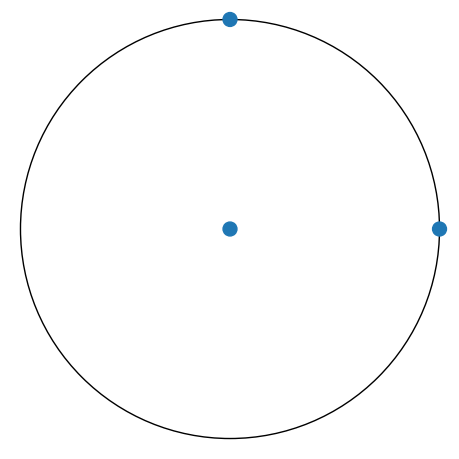
The spherical coordinates \((\phi, \theta)\) can be viewed while moving the cursor over the equatorial plane when plotting interactively (with qt5, notebook, or similar backends).
We can return the figure to save it or continue building upon it by passing return_figure=True
[3]:
temp_dir = tempfile.mkdtemp() + "/"  # Write to a temporary directory
vector_file = temp_dir + "vectors.png"
fig0 = v1.scatter(c=["r", "g", "b"], return_figure=True)
fig0.savefig(vector_file, bbox_inches="tight", pad_inches=0)
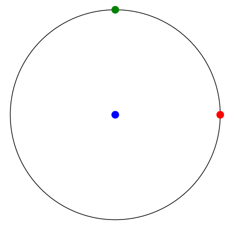
From Matplotlib with StereographicPlot.scatter()
[4]:
fig, ax = plt.subplots(subplot_kw={"projection": "stereographic"})
ax.scatter(v1, c=["r", "g", "b"])
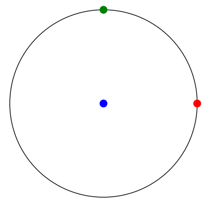
As usual with Matplotlib, the figure axes can be obtained from the returned figure
[5]:
fig0.axes[0]
[5]:
<StereographicPlot: >
Let’s turn on the azimuth \(\phi\) and polar \(\theta\) grid by updating the Matplotlib preferences
[6]:
plt.rcParams["axes.grid"] = True
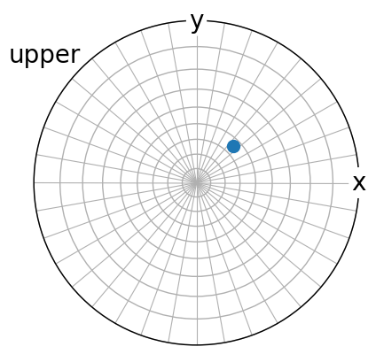
Upper and/or lower hemisphere#
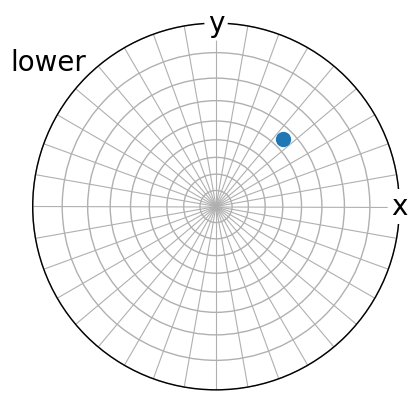
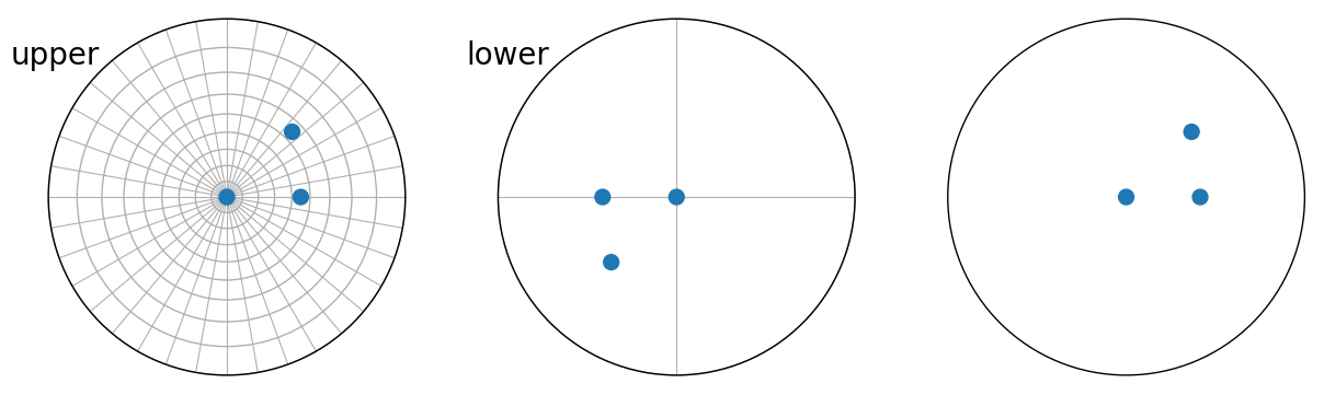
We can plot vectors impinging on the upper hemisphere and/or the lower hemisphere by passing “upper”, “lower”, or “both” to the hemisphere parameter in Vector3d.scatter()
[7]:
v2 = Vector3d([[1, 1, 2], [1, 1, -1]])
fig_kwargs = {"figsize": (5, 5)}
labels = ["x", "y", None]
v2.scatter(
axes_labels=labels, show_hemisphere_label=True, figure_kwargs=fig_kwargs
) # default hemisphere is "upper"
v2.scatter(
hemisphere="lower",
axes_labels=labels,
show_hemisphere_label=True,
figure_kwargs=fig_kwargs,
)
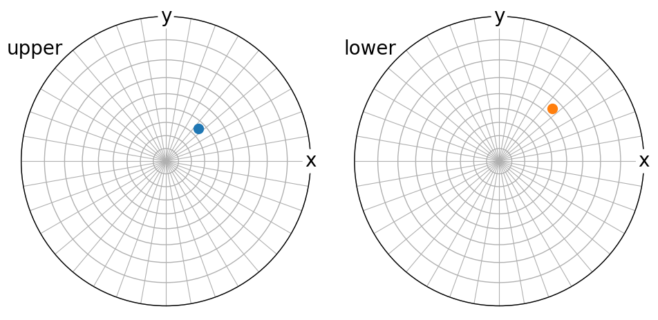
v2.scatter(hemisphere="both", axes_labels=labels, c=["C0", "C1"])
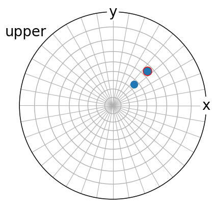
When reproject=True, vectors impinging on the opposite hemisphere are reprojected onto the visible hemisphere after reflection in the projection plane.
[8]:
reproject_scatter_kwargs = {"marker": "o", "fc": "None", "ec": "r", "s": 150}
v2.scatter(
    axes_labels=labels,
    show_hemisphere_label=True,
    figure_kwargs=fig_kwargs,
    reproject=True,
    reproject_scatter_kwargs=reproject_scatter_kwargs,
)
/home/docs/checkouts/readthedocs.org/user_builds/orix/conda/stable/lib/python3.11/site-packages/orix/plot/stereographic_plot.py:247: UserWarning: You passed both c and facecolor/facecolors for the markers. c has precedence over facecolor/facecolors. This behavior may change in the future.
  super().scatter(x, y, c=c, s=s, **updated_kwargs)
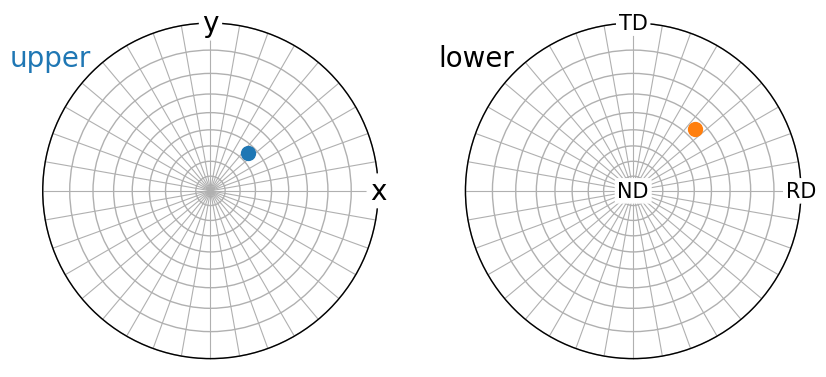
From Matplotlib by setting the StereographicPlot.hemisphere attribute. Remember to set the hemisphere before calling scatter()
[9]:
fig, ax = plt.subplots(ncols=2, subplot_kw={"projection": "stereographic"})

ax[0].scatter(v2, c="C0")  # blue
ax[0].show_hemisphere_label(color="C0")
ax[0].set_labels(zlabel=None)

ax[1].hemisphere = "lower"  # or "upper"
ax[1].scatter(v2, c="C1")  # orange
ax[1].show_hemisphere_label()
ax[1].set_labels("RD", "TD", "ND", size=15)
Control grid#
Whether to show the grid or not can be set globally via Matplotlib rcParams as we did above, or controlled via the parameters grid, True/False, and grid_resolution, a tuple with (azimuth, polar) resolution in degrees, to Vector3d.scatter(). Default grid resolution is \(10^{\circ}\) for both grids.
These can also be set after the figure is created by returning the figure
[11]:
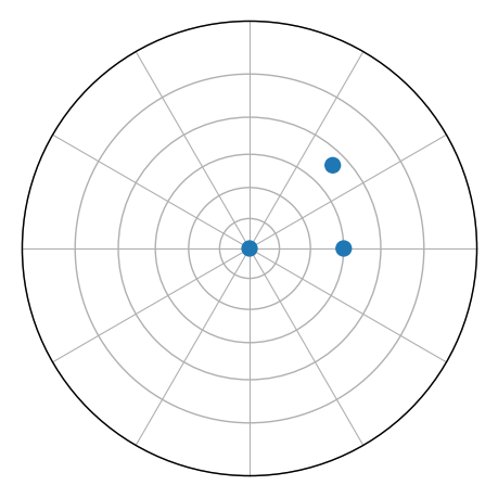
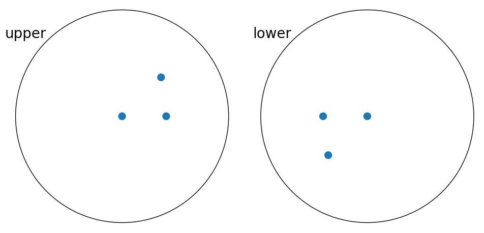
We can also remove the grid if desirable
[12]:
v4.scatter(hemisphere="both", grid=False)
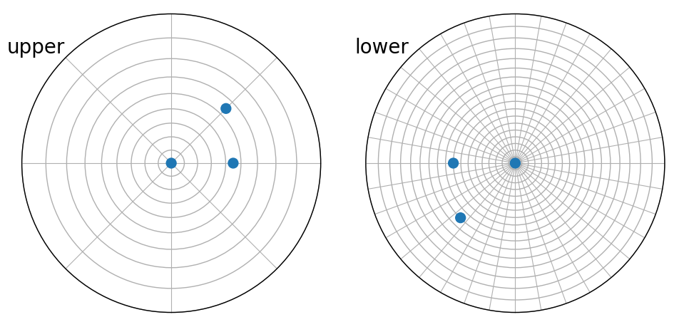
From Matplotlib, the polar and azimuth grid resolution can be set either upon axis initialization or after the axis is created using StereographicPlot.stereographic_grid()
[13]:
subplot_kw = {
    "projection": "stereographic",
    "polar_resolution": 10,
    "azimuth_resolution": 10,
}
fig, ax = plt.subplots(ncols=3, figsize=(15, 20), subplot_kw=subplot_kw)

ax[0].scatter(v4)
ax[0].show_hemisphere_label()

ax[1].hemisphere = "lower"
ax[1].show_hemisphere_label()
ax[1].scatter(v4)
ax[1].stereographic_grid(azimuth_resolution=90, polar_resolution=90)

ax[2].scatter(v4)
ax[2].stereographic_grid(False)
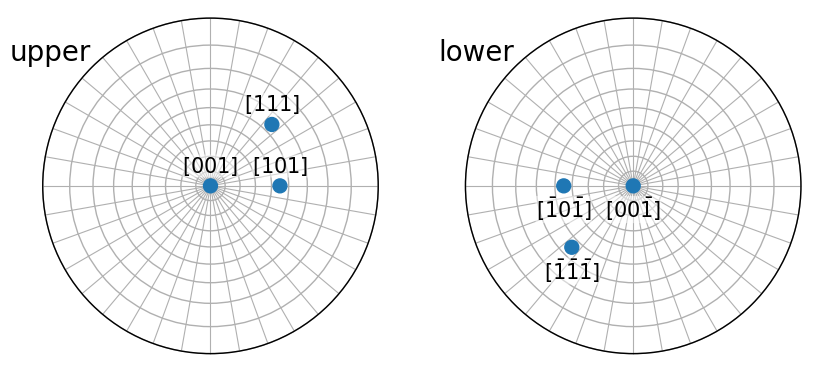
Annotate vectors#
Vectors can be annotated by passing a list of strings to the vector_labels parameter in Vector3d.scatter()
[14]:
v4.scatter(
    hemisphere="both",
    vector_labels=[str(vi).replace(" ", "") for vi in v4.data],
    text_kwargs={"size": 15, "offset": (0, 0.05)},
)
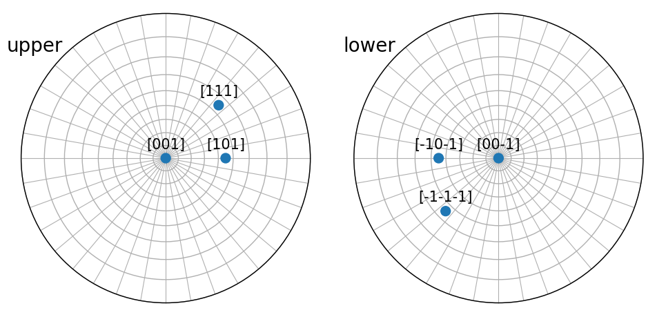
If we have integer vectors, like here, we can get nicely formatted labels using plot.format_labels().
[15]:
labels = plot.format_labels(v4.data, brackets=("[", "]"))
From Matplotlib, by looping over the vectors and adding text markers using StereographicPlot.text()
[16]:
fig, ax = plt.subplots(ncols=2, subplot_kw={"projection": "stereographic"})

ax[1].hemisphere = "lower"
ax[0].show_hemisphere_label()
ax[1].show_hemisphere_label()
ax[0].scatter(v4)
ax[1].scatter(v4)

bbox = {"boxstyle": "round,pad=0", "ec": "none", "fc": "w", "alpha": 0.5}
for i in range(v4.size):
    ax[0].text(v4[i], s=labels[i], size=15, offset=(0, 0.05), bbox=bbox)
    ax[1].text(
        v4[i], s=labels[i], size=15, va="top", offset=(0, -0.06), bbox=bbox
    )
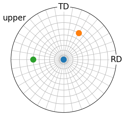
Pass spherical coordinates#
We can pass azimuth \(\phi\) and polar \(\theta\) angles instead of passing vectors. This only works in the “from Matplotlib” way
[17]:
fig = plt.figure(figsize=(5, 5))
ax = fig.add_subplot(projection="stereographic")
azimuth = np.deg2rad([0, 60, 180])
polar = np.deg2rad([0, 60, 60])
ax.scatter(azimuth, polar, c=["C0", "C1", "C2"], s=200)
ax.set_labels("RD", "TD", None)
ax.show_hemisphere_label()

Here, we also passed None to StereographicPlot.set_labels() so that the Z axis label is not shown.
Producing the exact same plot with Vector3d.scatter()
[18]:
Vector3d.from_polar(azimuth=azimuth, polar=polar).scatter(
    axes_labels=["RD", "TD", None],
    show_hemisphere_label=True,
    figure_kwargs={"figsize": (5, 5)},
    c=["C0", "C1", "C2"],
    s=200,
)
Draw great and small circles#
We can draw the trace of a plane perpendicular to a vector using Vector3d.draw_circle()
[19]:
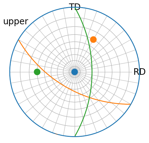
Let’s also add the vector perpendicular to the last two vectors and its great circle. We can add to the previous figure by passing the returned figure into the figure parameter in Vector3d.scatter() and Vector3d.draw_circle()
[20]:
[20]:
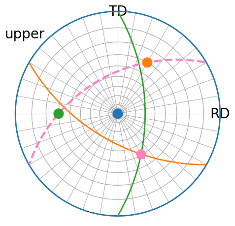
From Matplotlib using StereograhicPlot.draw_circle(), also showing a small circle (not perpendicular, but at a \(45^{\circ}\) angle in this case)
[21]:
fig = plt.figure(figsize=(5, 5))
ax = fig.add_subplot(projection="stereographic")
colors = ["C0", "C1", "C2"]
azimuth = np.deg2rad([0, 60, 180])
polar = np.deg2rad([0, 60, 60])
ax.scatter(azimuth, polar, c=colors, s=200)
ax.set_labels("RD", "TD", None)
ax.show_hemisphere_label()
ax.draw_circle(azimuth, polar, color=colors, linewidth=2)

# Let's also add the vector perpendicular to the last two vectors and its
# great circle
v6 = Vector3d.from_polar(azimuth=azimuth[1:], polar=polar[1:])
v7 = v6[0].cross(v6[1])
ax.scatter(v7, c="xkcd:pink", marker="p", s=250)
ax.draw_circle(
    v7,
    color="xkcd:pink",
    linestyle="--",
    linewidth=3,
    opening_angle=0.25 * np.pi,
)
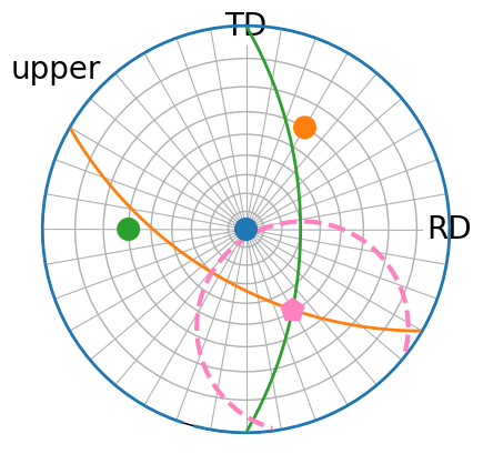
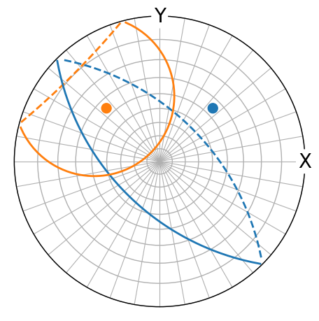
We can also draw the part of the circles only visible on the other hemisphere by passing reproject=True
[22]:
v8 = Vector3d([(1, 1, 1), (-1, 1, 1)])
fig = v8.scatter(axes_labels=["X", "Y"], return_figure=True, c=["C0", "C1"])
v8.draw_circle(
    reproject=True,
    figure=fig,
    color=["C0", "C1"],
    opening_angle=np.deg2rad([90, 45]),
)