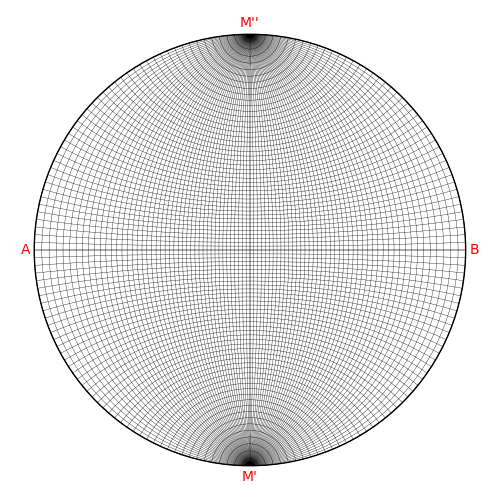
Wulff net

This example shows how to draw a customized Wulff net in stereographic plots using wulff_net()

import matplotlib.pyplot as plt

from orix.plot import register_projections
from orix.quaternion.symmetry import C6h

register_projections()  # Register our custom Matplotlib projections

Plot two stereographic projections, one with the standard Wulff net, another with a customized net

fig = plt.figure(figsize=(6, 4), layout="tight")
ax0 = fig.add_subplot(121, projection="stereographic")
ax1 = fig.add_subplot(122, projection="stereographic")

# Display a standard Wulff net with 2 degree minor markers and 10 degree
# major markers, with 10 degree caps at the tops and bottoms.
ax0.set_title("Standard Wulff net")
ax0.wulff_net()

# The grid spacing can also be changed or turned on and off, similar to
# matplotlib.axes.Axes.grid(). Here, the latitudinal grid is set to 3
# degrees (15 degrees for major grid lines), and the longitudinal to 9
# degrees (45 degrees for major grid lines).
ax1.set_title("Custom Wulff net")
ax1.wulff_net(True, 3, 9, 15, 45, 15)

# Turn it off
ax1.wulff_net()

# Then turn it back on, with the previously defined grid spacing saved.
ax1.wulff_net()

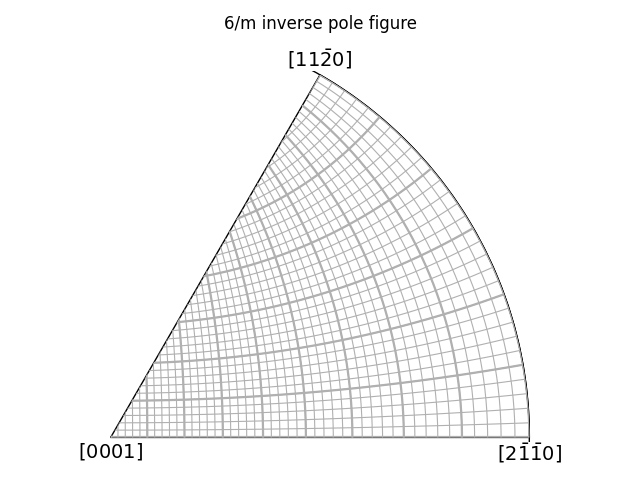
The net also displays nicely for inverse pole figures (stereographic projections restricted to a fundamental sector)

fig = plt.figure(layout="tight")
ax = fig.add_subplot(projection="ipf", symmetry=C6h)

ax.wulff_net()
ax.set_title(f"{C6h.name} inverse pole figure", pad=30)

plt.show()

Estimated memory usage: 493 MB