This page was generated from doc/tutorials/crystal_directions.ipynb. Interactive online version: .

Crystal directions

In this tutorial we will perform operations with and plot directions with respect to the crystal reference frame \((\mathbf{e}_1, \mathbf{e}_2, \mathbf{e}_3)\) using Miller indices with the orix.vector.Miller class.

Many of the initial examples, explaining basic crystallographic computations with crystal lattice directions \([uvw]\) and crystal lattice planes \((hkl)\), are taken from the textbook Introduction to Conventional Transmission Electron Microscopy ([De Graef, 2003]). Some of the later examples are also inspired by MTEX’ excellent documentation on Miller indices and operations with them.

%matplotlib inline

from diffpy.structure import Lattice, Structure
import matplotlib.pyplot as plt
import numpy as np

from orix import plot
from orix.crystal_map import Phase
from orix.quaternion import Orientation, Rotation, symmetry
from orix.vector import Miller, Vector3d


plt.rcParams.update(
    {
        "figure.figsize": (7, 7),
        "font.size": 20,
        "axes.grid": True,
        "lines.markersize": 10,
        "lines.linewidth": 2,
    }
)

To start with, let’s create a tetragonal crystal with lattice parameters \(a\) = \(b\) = 0.5 nm and \(c\) = 1 nm and symmetry elements described by point group \(S = 4\)

tetragonal = Phase(
    point_group="4",
    structure=Structure(lattice=Lattice(0.5, 0.5, 1, 90, 90, 90)),
)
print(tetragonal)
print(tetragonal.structure.lattice)

<name: . space group: None. point group: 4. proper point group: 4. color: tab:blue>
Lattice(a=0.5, b=0.5, c=1, alpha=90, beta=90, gamma=90)

Here, the Phase class attaches a point group symmetry, Symmetry, to a Structure containing a Lattice (where the crystal axes are defined), and possibly some Atoms.

Directions \([uvw]\)

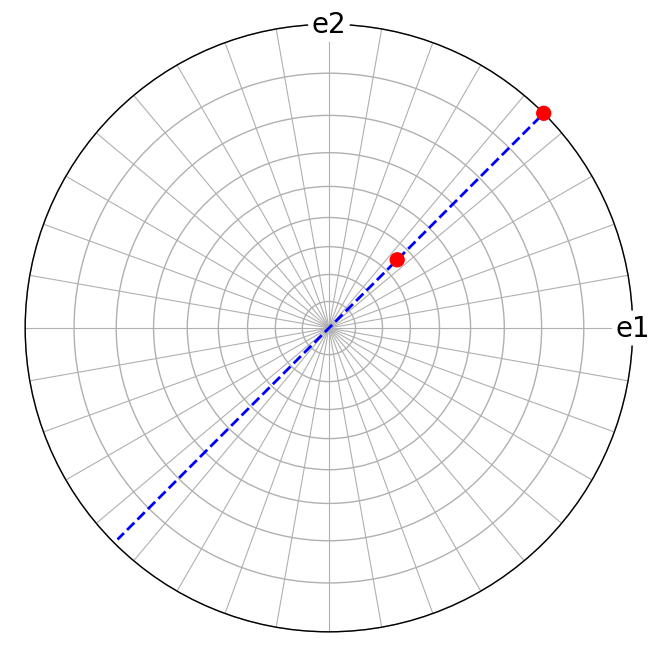
A crystal lattice direction \(\mathbf{t} = u \cdot \mathbf{a} + v \cdot \mathbf{b} + w \cdot \mathbf{c}\) is a vector with coordinates \((u, v, w)\) with respect to the crystal axes \((\mathbf{a}, \mathbf{b}, \mathbf{c})\), and is denoted \([uvw]\). We can create a set of these Miller indices by passing a list/array/tuple to uvw in Miller

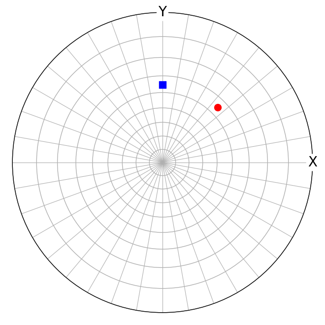
t1 = Miller(uvw=[[1, 2, 0], [3, 1, 1]], phase=tetragonal)
t1.scatter(c=["b", "r"], axes_labels=["e1", "e2"])
t1

Miller (2,), point group 4, uvw
[[1. 2. 0.]
 [3. 1. 1.]]

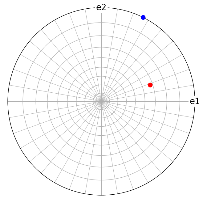
Here, we plotted the lattice directions \(\mathbf{t}_i\) in the stereographic projection using the Vector3d.scatter() plotting method. This also works for Miller.scatter() since the Miller class inherits most of the functionality in the Vector3d class.

Let’s compute the dot product in nanometres and the angle in degrees between the vectors

t1[0].dot(t1[1])

array([1.25])

t1[0].angle_with(t1[1], degrees=True)

array([53.3007748])

The length of a direct lattice vector \(|\mathbf{t}|\) is available via the Miller.length property, given in lattice parameter units (nm in this case)

Miller(uvw=[0, -0.5, 0.5], phase=tetragonal).length

array([0.55901699])

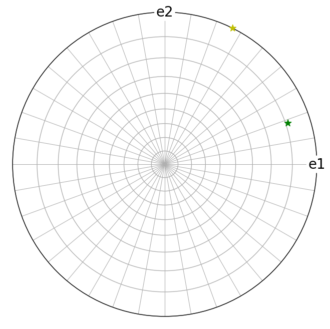
Planes \((hkl)\)

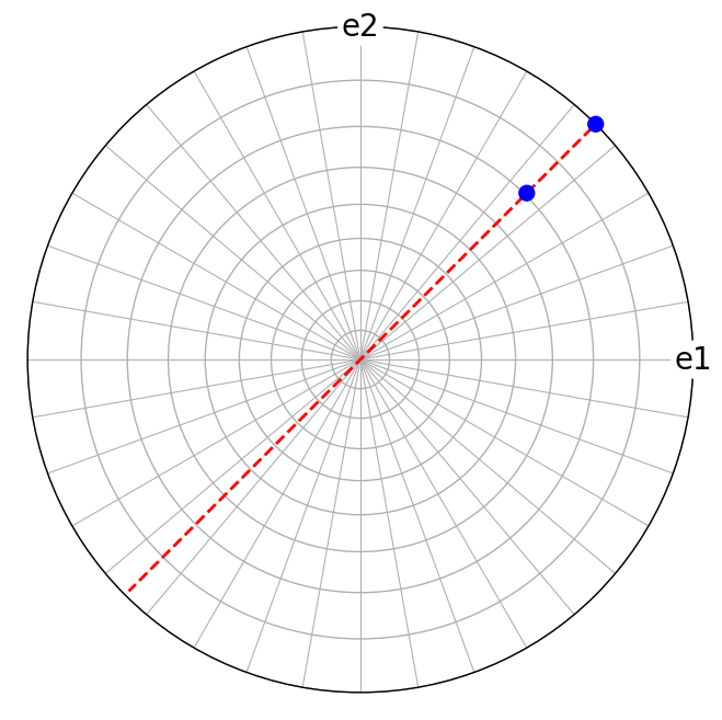
A crystal lattice plane \((hkl)\) is described by its normal vector \(\mathbf{g} = h\cdot\mathbf{a^*} + k\cdot\mathbf{b^*} + l\cdot\mathbf{c^*}\), where \((\mathbf{a^*}, \mathbf{b^*}, \mathbf{c^*})\) are the reciprocal crystal axes. As for crystal directions \([uvw]\), we can create a set of these Miller indices by passing hkl instead of uvw to Miller

g1 = Miller(hkl=t1.uvw, phase=tetragonal)
g1.scatter(c=["y", "g"], marker="*", axes_labels=["e1", "e2"])
g1

Miller (2,), point group 4, hkl
[[1. 2. 0.]
 [3. 1. 1.]]

Let’s compute the angle in degrees between the lattice plane normals

g1[0].angle_with(g1[1], degrees=True)

array([45.69879831])

Note that the lattice plane normals \((hkl)\) are not always parallel to the lattice directions \([uvw]\), even if the indices are the same

fig = t1.scatter(return_figure=True, c=["b", "r"])
g1.scatter(figure=fig, c=["y", "g"], marker="*", axes_labels=["e1", "e2"])

We can get the reciprocal components of the lattice vector \(\mathbf{t}\) = [114] (i.e. which lattice plane the [114] direction is perpendicular to) by accessing Miller.hkl for a Miller object with crystal directions (or Miller.uvw for a Miller object with crystal plane normals)

Miller(uvw=[1, 1, 4], phase=tetragonal).hkl

array([[0.25, 0.25, 4.  ]])

We see that the lattice vector \(\mathbf{t}\) = [114] is perpendicular to the lattice plane \(\mathbf{g}\) = (1 1 16).

The length of reciprocal lattice vectors can also be accessed via the Miller.length property. The length equals \(|\mathbf{g}| = \frac{1}{d_{\mathrm{hkl}}}\) in reciprocal lattice parameter units (nm^-1 in this case)

g1.length

array([4.47213595, 6.40312424])

We can then obtain the interplanar spacing \(d_{\mathrm{hkl}}\)

1 / g1.length

array([0.2236068 , 0.15617376])

Zone axes

The cross product \(\mathbf{g} = \mathbf{t}_1 \times \mathbf{t}_2\) of the lattice vectors \(\mathbf{t}_1\) = [110] and \(\mathbf{t}_2\) = [111] in the tetragonal crystal, in direct space, is described by a vector expressed in reciprocal space, \((hkl)\)

t2 = Miller(uvw=[[1, 1, 0], [1, 1, 1]], phase=tetragonal)
g2 = t2[0].cross(t2[1])
g2

Miller (1,), point group 4, hkl
[[ 0.25 -0.25  0.  ]]

The exact “indices” are returned. However, we can get a new Miller instance with the indices rounded down or up to the closest smallest integer via the Miller.round() method

g2.round()

Miller (1,), point group 4, hkl
[[ 1. -1.  0.]]

The maximum index that Miller.round() may return can be set by passing the max_index parameter.

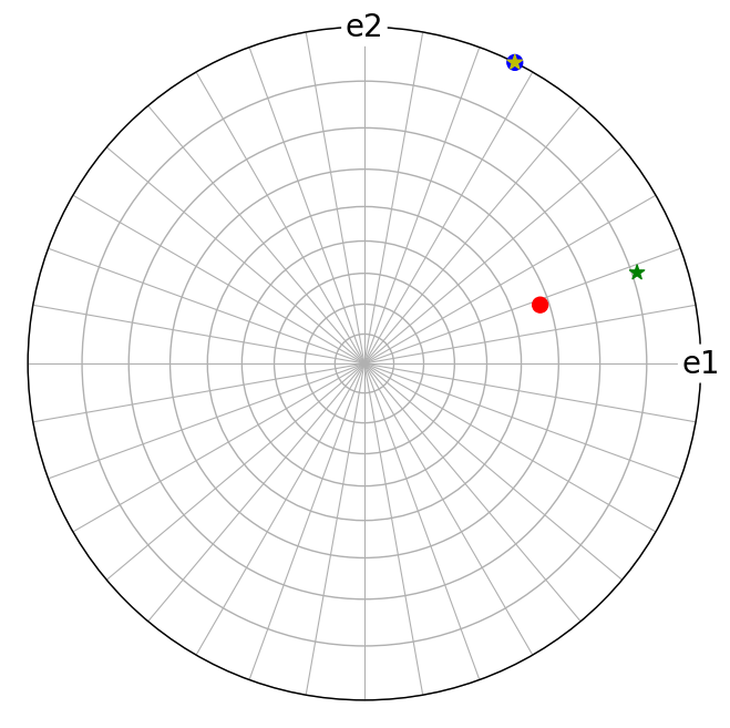
We can plot these direct lattice vectors \([uvw]\) and the vectors normal to the cross product vector, i.e. normal to the reciprocal lattice vector \((hkl)\)

fig = t2.scatter(return_figure=True, c="r", axes_labels=["e1", "e2"])
g2.draw_circle(figure=fig, color="b", linestyle="--")

Likewise, the cross product of reciprocal lattice vectors \(\mathbf{g}_1\) = (110) and \(\mathbf{g}_2\) = (111) results in a direct lattice vector

g3 = Miller(hkl=t2.uvw, phase=tetragonal)
t3 = g3[0].cross(g3[1]).round()
t3

Miller (1,), point group 4, uvw
[[ 1. -1.  0.]]

fig = g3.scatter(return_figure=True, c="b", axes_labels=["e1", "e2"])
t3.draw_circle(figure=fig, color="r", linestyle="--")

Trigonal and hexagonal index conventions

Crystal lattice vectors and planes in lattices with trigonal and hexagonal crystal symmetry are typically expressed in Weber symbols \(\mathbf{t} = [UVTW]\) and Miller-Bravais indices \(\mathbf{g} = (hkil)\). The definition of \([UVTW]\) used in orix follows Introduction to Conventional Transmission Electron Microscopy (DeGraef, 2003)

\begin{align} U &= \frac{2u - v}{3},\\ V &= \frac{2v - u}{3},\\ T &= -\frac{u + v}{3},\\ W &= w. \end{align}

For a plane, the \(h\), \(k\), and \(l\) indices are the same in \((hkl)\) and \((hkil)\), and \(i = -(h + k)\).

The first three Miller indices always sum up to zero, i.e.

\begin{align} U + V + T &= 0,\\ h + k + i &= 0. \end{align}

trigonal = Phase(
    point_group="321",
    structure=Structure(lattice=Lattice(4.9, 4.9, 5.4, 90, 90, 120)),
)
trigonal

<name: . space group: None. point group: 321. proper point group: 32. color: tab:blue>

t4 = Miller(UVTW=[2, 1, -3, 1], phase=trigonal)
t4

Miller (1,), point group 321, UVTW
[[ 2.  1. -3.  1.]]

g4 = Miller(hkil=[1, 1, -2, 3], phase=trigonal)
g4

Miller (1,), point group 321, hkil
[[ 1.  1. -2.  3.]]

t4.scatter(c="C0", grid_resolution=(30, 30), axes_labels=["e1", "e2"])
g4.scatter(figure=plt.gcf(), c="C1")

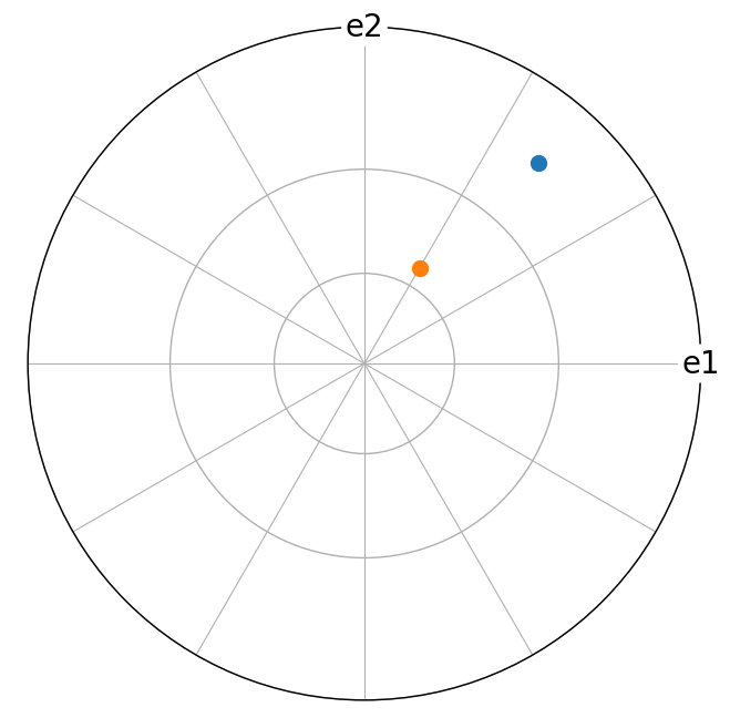
We can switch between the coordinate format of a vector. However, this does not change the vector, since all vectors are stored with respect to the cartesian coordinate system internally.

print(g4, "\n\n", g4.data)

Miller (1,), point group 321, hkil
[[ 1.  1. -2.  3.]]

 [[0.20408163 0.35347976 0.55555556]]

g4.coordinate_format = "UVTW"
print(g4, "\n\n", g4.data)

Miller (1,), point group 321, UVTW
[[ 0.0278  0.0278 -0.0555  0.1029]]

 [[0.20408163 0.35347976 0.55555556]]

Getting the closest integer indices, however, changes the vector

g4_round = g4.round()
print(g4_round, "\n\n", g4_round.data)

Miller (1,), point group 321, UVTW
[[ 3.  3. -6. 11.]]

 [[22.05       38.19172031 59.4       ]]

Symmetrically equivalent directions and planes

The symmetry operations \(s\) of the point group symmetry assigned to a crystal lattice can be applied to describe symmetrically equivalent crystal directions and planes. This applies to crystals in all seven systems (triclinic, monoclinic, orthorhombic, trigonal, tetragonal, hexagonal, and cubic), but we’ll use the cubic crystal as an example because of its high symmetry

cubic = Phase(point_group="m-3m")
print(cubic, "\n", cubic.structure.lattice.abcABG())

<name: . space group: None. point group: m-3m. proper point group: 432. color: tab:blue>
 (1.0, 1.0, 1.0, 90.0, 90.0, 90.0)

The directions \(\mathbf{t}\) parallel to the crystal axes (\(\mathbf{a}\), \(\mathbf{b}\), \(\mathbf{c}\)) given by \([100]\), \([\bar{1}00]\), \([010]\), \([0\bar{1}0]\), \([001]\), and \([00\bar{1}]\) (\(\bar{1}\) means “-1”) are symmetrically equivalent, and can be obtained using Miller.symmetrise()

t100 = Miller(uvw=[1, 0, 0], phase=cubic)
t100.symmetrise(unique=True)

Miller (6,), point group m-3m, uvw
[[ 1.  0.  0.]
 [ 0.  1.  0.]
 [-1.  0.  0.]
 [ 0. -1.  0.]
 [ 0.  0.  1.]
 [ 0.  0. -1.]]

Without passing unique=True, since the cubic crystal symmetry is described by 48 symmetry operations \(s\) (or elements), 48 directions \(\mathbf{t}\) would have been returned.

The six symmetrically equivalent directions, known as a family, may be expressed collectively as \(\left<100\right>\), the brackets implying all six permutations or variants of 1, 0, 0. This particular family is said to have a multiplicity of 6

t100.multiplicity

array([6])

t6 = Miller(uvw=[[1, 0, 0], [1, 1, 0], [1, 1, 1]], phase=cubic)
t6

Miller (3,), point group m-3m, uvw
[[1. 0. 0.]
 [1. 1. 0.]
 [1. 1. 1.]]

t6.multiplicity

array([ 6, 12,  8])

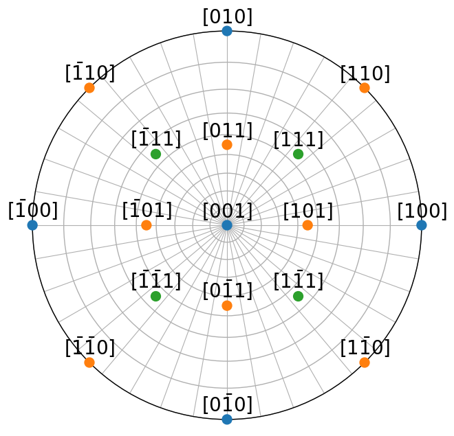
Let’s plot the symmetrically equivalent directions from the direction families \(\left<100\right>\), \(\left<110\right>\), and \(\left<111\right>\) impinging on the upper hemisphere. By also returning the indices of which family each symmetrically equivalent direction belongs to from Miller.symmetrise(), we can give a unique color per family.

t7, idx = t6.symmetrise(unique=True, return_index=True)
labels = plot.format_labels(t7.uvw, ("[", "]"))

# Get an array with one color per family of vectors
colors = np.array([f"C{i}" for i in range(t6.size)])[idx]

t7.scatter(c=colors, vector_labels=labels, text_kwargs={"offset": (0, 0.02)})

Similarly, symmetrically equivalent planes \(\mathbf{g} = (hkl)\) can be collectively expressed as planes of the form \(\{hkl\}\)

g5 = Miller(hkl=[[1, 0, 0], [1, 1, 0], [1, 1, 1]], phase=cubic)
g5.multiplicity

array([ 6, 12,  8])

g6, idx = g5.symmetrise(unique=True, return_index=True)

labels = plot.format_labels(g6.hkl, ("(", ")"))
colors = np.array([f"C{i}" for i in range(g5.size)])[idx]

g6.scatter(c=colors, vector_labels=labels, text_kwargs={"offset": (0, 0.02)})

We computed the angles between directions and plane normals earlier in this tutorial. In general, Miller.angle_with() does not consider symmetrically equivalent directions, unless use_symmetry=True is passed. Consider \((100)\) and \((\bar{1}00)\) and \((111)\) and \((\bar{1}11)\) in the stereographic plot above

g7 = Miller(hkl=[[1, 0, 0], [1, 1, 1]], phase=cubic)
g8 = Miller(hkl=[[-1, 0, 0], [-1, 1, 1]], phase=cubic)

g7.angle_with(g8, degrees=True)

array([180.        ,  70.52877937])

g7.angle_with(g8, use_symmetry=True, degrees=True)

array([0., 0.])

Thus, passing use_symmetry=True ensures that the smallest angles between \(\mathbf{g}_1\) and the symmetrically equivalent directions to \(\mathbf{g}_2\) are found.

Directions and planes in rotated crystals

Let’s consider the orientation of a cubic crystal rotated \(45^{\circ}\) about the sample \(\mathbf{Z}\) axis. This orientation is denoted \((\hat{\mathbf{n}}, \omega)\) = \(([001], -45^{\circ})\) in axis-angle notation (see discussion by [Rowenhorst et al., 2015]). Orientations in orix are interpreted as basis transformations from the sample to the crystal (so-called “lab2crystal”). We therefore have to invert the orientation to get a crystal direction or plane normal expressed in the sample reference frame.

O = Orientation.from_axes_angles(
    [0, 0, 1], -45, cubic.point_group, degrees=True
)
O

Orientation (1,) m-3m
[[ 0.9239 -0.     -0.     -0.3827]]

We can apply this orientation to a crystal direction \(\mathbf{t} = [uvw]\) to find this direction in this particular crystal with respect to the sample coordinate system, denoted \(\mathbf{v} = O^{-1} \cdot \mathbf{t}\)

t8 = Miller(uvw=[1, 1, 1], phase=cubic)
v = Vector3d(~O * t8)
v

Vector3d (1,)
[[-0.      1.4142  1.    ]]

# [uvw] in unrotated crystal with orientation the identity orientation
fig = t8.scatter(c="r", return_figure=True, axes_labels=["X", "Y"])

# [uvw] in rotated crystal with (n, omega) = ([001], -45 deg)
(~O * t8).scatter(figure=fig, c="b", marker="s")

We see that the \([111]\) vector in the rotated crystal with orientation \(O = (\hat{\mathbf{n}}, \omega) = ([001], -45^{\circ})\) lies in the sample Y-Z plane.

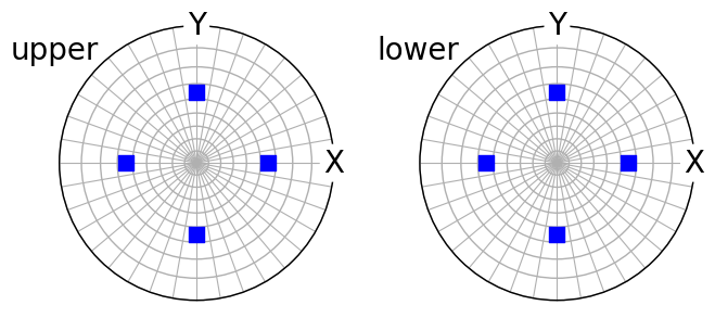
We can apply all cubic crystal symmetry operations \(s_i\) to obtain the coordinates with respect to the sample reference frame for all crystallographically equivalent, but unique, directions, \(\mathbf{v} = O^{-1} \cdot (s_i \cdot \mathbf{t} \cdot s_i^{-1})\)

(~O * t8.symmetrise(unique=True)).scatter(
    c="b", marker="s", axes_labels=["X", "Y"], hemisphere="both"
)

The same applied to a trigonal crystal direction

O2 = Orientation.from_euler([10, 20, 30], trigonal.point_group, degrees=True)
O2

Orientation (1,) 321
[[ 0.9254 -0.171   0.0302 -0.3368]]

g9 = Miller(hkil=[1, -1, 0, 0], phase=trigonal)
g9

Miller (1,), point group 321, hkil
[[ 1. -1. -0.  0.]]

v2 = ~O2 * g9.symmetrise(unique=True)
v2.scatter(
    hemisphere="both",
    grid_resolution=(30, 30),
    figure_kwargs=dict(figsize=(10, 5)),
    axes_labels=["X", "Y"],
)

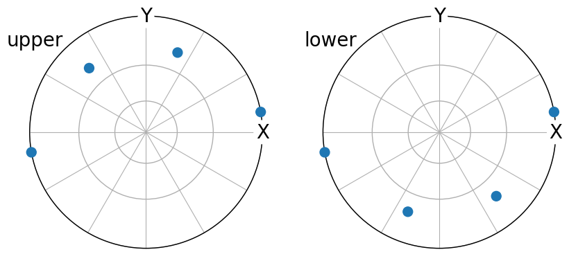
The stereographic plots above are essentially the \(\mathbf{g} = \{1\bar{1}00\}\) pole figure representation of the orientation \(O_2\).

---

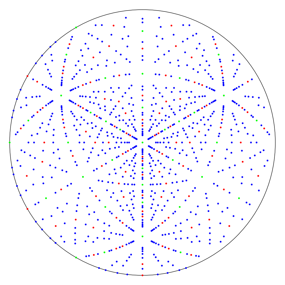
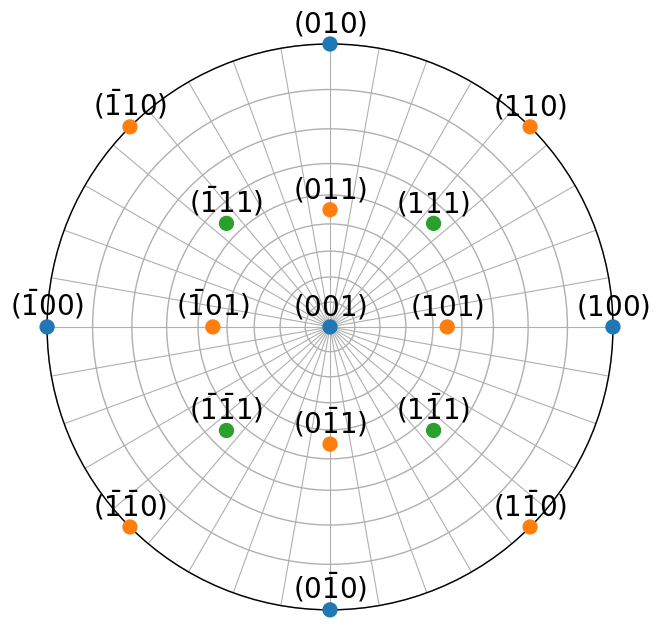
A diamond [111] pole figure

Let’s make a pole figure in the \(\mathbf{t}\) = [111] direction of the diamond structure, as seen in this figure from Wikipedia.

The figure caption reads as follows

The spots in the stereographic projection show the orientation of lattice planes with the 111 in the center. Only poles for a non-forbidden Bragg reflection are shown between Miller indices -10 <= (h,k,l) <= 10. The green spots contain Miller indices up to 3, for example 111, 113, 133, 200 etc in its fundamental order. Red are those raising to 5, ex. 115, 135, 335 etc, while blue are all remaining until 10, such as 119, 779, 10.10.00 etc.

diamond = Phase(space_group=227)
t = Miller.from_highest_indices(phase=diamond, uvw=[10, 10, 10])
t

Miller (9260,), point group m-3m, uvw
[[ 10.  10.  10.]
 [ 10.  10.   9.]
 [ 10.  10.   8.]
 ...
 [-10. -10.  -8.]
 [-10. -10.  -9.]
 [-10. -10. -10.]]

Remove duplicates under symmetry using Miller.unique()

t2 = t.unique(use_symmetry=True)
t2.size

285

Symmetrise to get all symmetrically equivalent directions

t3 = t2.symmetrise(unique=True)
t3

Miller (9260,), point group m-3m, uvw
[[  1.   0.   0.]
 [  0.   1.   0.]
 [ -1.   0.   0.]
 ...
 [ 10.  10. -10.]
 [-10.  10. -10.]
 [-10. -10. -10.]]

Remove forbidden reflections in face-centered cubic structures (all hkl must be all even or all odd)

selection = np.sum(np.mod(t3.hkl, 2), axis=1)
allowed = np.array([i not in [1, 2] for i in selection], dtype=bool)
t4 = t3[allowed]
t4

Miller (2330,), point group m-3m, uvw
[[  2.   0.   0.]
 [  0.   2.   0.]
 [ -2.   0.   0.]
 ...
 [ 10.  10. -10.]
 [-10.  10. -10.]
 [-10. -10. -10.]]

Assign colors to each class of vectors as per the description on Wikipedia

uvw = np.abs(t4.uvw)
green = np.all(uvw <= 3, axis=-1)
red = np.any(uvw > 3, axis=-1) * np.all(uvw <= 5, axis=-1)
blue = np.any(uvw > 5, axis=-1)
rgb_mask = np.column_stack([red, green, blue])

# Sanity check
print(np.count_nonzero(rgb_mask) == t4.size)

True

Rotate directions so that [111] impinges the unit sphere in the north pole (out of plane direction)

vz = Vector3d.zvector()
v111 = Vector3d([1, 1, 1])
R1 = Rotation.from_axes_angles(vz.cross(v111), -vz.angle_with(v111))
R2 = Rotation.from_axes_angles(vz, -15, degrees=True)
t5 = R2 * R1 * t4

Restrict to upper hemisphere and remove duplicates

is_upper = t5.z > 0
t6 = t5[is_upper]
rgb_mask2 = rgb_mask[is_upper]

_, idx = t6.unit.unique(return_index=True)
t7 = t6[idx]
rgb_mask2 = rgb_mask2[idx]

Finally, plot the vectors

rgb = np.zeros_like(t7.uvw)
rgb[rgb_mask2] = 1

t7.scatter(c=rgb, s=10, grid=False, figure_kwargs=dict(figsize=(12, 12)))