This page was generated from doc/tutorials/clustering_orientations.ipynb. Interactive online version: .

Clustering orientations

In this tutorial we will cluster Ti crystal orientations using data obtained from a highly deformed specimen, using EBSD, as presented in [Johnstone et al., 2020]. The data can be downloaded to your local cache via the orix.data module.

Import orix classes and various dependencies

# Exchange inline for notebook (or qt5 from pyqt) for interactive plotting
%matplotlib inline

# Import core external
import numpy as np
import matplotlib.pyplot as plt
from sklearn.cluster import DBSCAN

# Colorisation and visualisation
from matplotlib.colors import to_rgb
from mpl_toolkits.mplot3d.art3d import Line3DCollection
from matplotlib.lines import Line2D
from skimage.color import label2rgb

# Import orix classes
from orix import data, plot
from orix.quaternion import Orientation, OrientationRegion, Rotation
from orix.quaternion.symmetry import D6
from orix.vector import AxAngle, Vector3d


plt.rcParams.update(
    {"font.size": 20, "figure.figsize": (10, 10), "figure.facecolor": "w"}
)

Import data

Load Ti orientations with the point group symmetry D6 (622). We have to explicitly allow downloading from an external source.

ori = data.ti_orientations(allow_download=True)
ori

Orientation (193167,) 622
[[ 0.3027  0.0869 -0.5083  0.8015]
 [ 0.3088  0.0868 -0.5016  0.8034]
 [ 0.3057  0.0818 -0.4995  0.8065]
 ...
 [ 0.4925 -0.1633 -0.668   0.5334]
 [ 0.4946 -0.1592 -0.6696  0.5307]
 [ 0.4946 -0.1592 -0.6696  0.5307]]

The orientations define transformations from the sample (lab) to the crystal reference frame, i.e. the Bunge convention. The above referenced paper assumes the opposite convention, which is the one used in MTEX. So, we have to invert the orientations

ori = ~ori

Reshape the orientation mapping data to the correct spatial dimension for the scan

ori = ori.reshape(381, 507)

Select a subset of the orientations to a suitable size for this demonstration

ori = ori[-100:, :200]

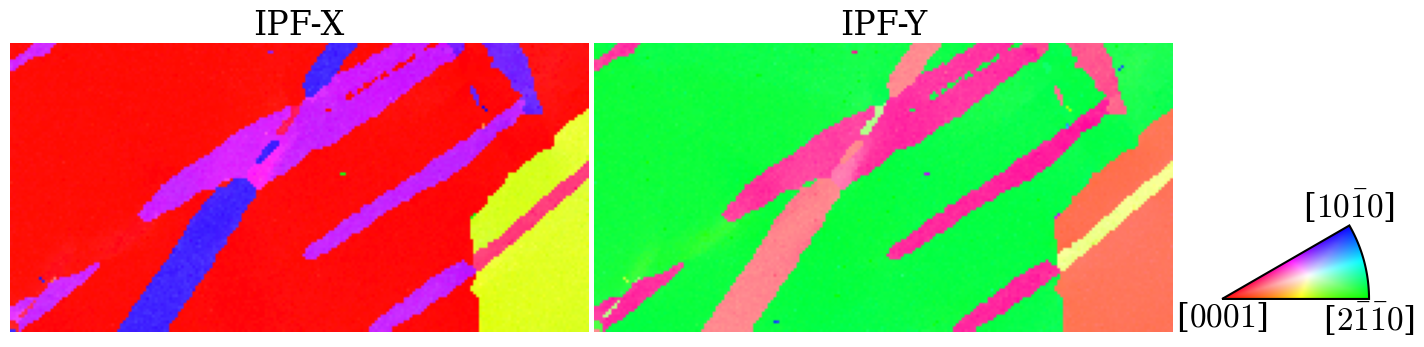
Get an overview of the orientations from orientation maps

ckey = plot.IPFColorKeyTSL(D6)

directions = [(1, 0, 0), (0, 1, 0)]
titles = ["X", "Y"]

fig, axes = plt.subplots(ncols=2, figsize=(15, 10))
for i, ax in enumerate(axes):
    ckey.direction = Vector3d(directions[i])
    # Invert because orix assumes lab2crystal when coloring orientations
    ax.imshow(ckey.orientation2color(~ori))
    ax.set_title(f"IPF-{titles[i]}")
    ax.axis("off")

# Add color key
ax_ipfkey = fig.add_axes(
    [0.932, 0.37, 0.1, 0.1],  # (Left, bottom, width, height)
    projection="ipf",
    symmetry=ori.symmetry.laue,
)
ax_ipfkey.plot_ipf_color_key()
ax_ipfkey.set_title("")
fig.subplots_adjust(wspace=0.01)

Map the orientations into the fundamental zone (find symmetrically equivalent orientations with the smallest angle of rotation) of D6

ori = ori.map_into_symmetry_reduced_zone()

Compute distance matrix

# Increase the chunk size for a faster but more memory intensive computation
D = ori.get_distance_matrix(lazy=True, chunk_size=20)

[########################################] | 100% Completed | 83.70 s

D = D.reshape(ori.size, ori.size)

Clustering

For parameter explanations of the DBSCAN algorithm (Density-Based Spatial Clustering for Applications with Noise), see the scikit-learn documentation.

# This call will use about 6 GB of memory, but the data precision of
# the D matrix can be reduced from float64 to float32 save memory:
D = D.astype(np.float32)

dbscan = DBSCAN(
    eps=0.05,  # Max. distance between two samples in radians
    min_samples=40,
    metric="precomputed",
).fit(D)

unique_labels, all_cluster_sizes = np.unique(
    dbscan.labels_, return_counts=True
)
print("Labels:", unique_labels)

all_labels = dbscan.labels_.reshape(ori.shape)
n_clusters = unique_labels.size - 1
print("Number of clusters:", n_clusters)

Labels: [-1  0  1  2  3  4  5  6]
Number of clusters: 7

Calculate the mean orientation of each cluster

unique_cluster_labels = unique_labels[
    1:
]  # Without the "no-cluster" label -1
cluster_sizes = all_cluster_sizes[1:]

q_mean = [ori[all_labels == l].mean() for l in unique_cluster_labels]
cluster_means = Orientation.stack(q_mean).flatten()

# Map into the fundamental zone
cluster_means.symmetry = D6
cluster_means = cluster_means.map_into_symmetry_reduced_zone()
cluster_means

Orientation (7,) 622
[[ 0.7093  0.1617 -0.6683 -0.1554]
 [ 0.8519  0.3835  0.3346 -0.1231]
 [ 0.8647  0.4319 -0.1888  0.1735]
 [ 0.8596  0.4059  0.2586 -0.1716]
 [ 0.785   0.2649  0.5591  0.0311]
 [ 0.7096  0.6541  0.2039  0.1642]
 [ 0.7942 -0.3078 -0.5239 -0.002 ]]

Inspect rotation axes in the axis-angle representation

cluster_means.axis

Vector3d (7,)
[[ 0.2293 -0.948  -0.2205]
 [ 0.7324  0.639  -0.2351]
 [ 0.8599 -0.3759  0.3454]
 [ 0.7944  0.5061 -0.3358]
 [ 0.4276  0.9026  0.0502]
 [ 0.9284  0.2895  0.2331]
 [-0.5065 -0.8622 -0.0033]]

Recenter data relative to the matrix cluster and recompute means

ori_recentered = (~cluster_means[0]) * ori

# Map into the fundamental zone
ori_recentered.symmetry = D6
ori_recentered = ori_recentered.map_into_symmetry_reduced_zone()

cluster_means_recentered = Orientation.stack(
    [ori_recentered[all_labels == l].mean() for l in unique_cluster_labels]
).flatten()
cluster_means_recentered

Orientation (7,) 1
[[ 1.      0.     -0.     -0.    ]
 [ 0.8464 -0.2653 -0.4618 -0.    ]
 [ 0.7824  0.3119  0.5391 -0.0007]
 [ 0.7932 -0.3012 -0.5292  0.0059]
 [ 0.9674 -0.1234 -0.2211  0.0051]
 [ 0.8606 -0.4344 -0.2657  0.0035]
 [ 0.9545 -0.2864 -0.0372 -0.0749]]

Inspect recentered rotation axes in the axis-angle representation

cluster_means_recentered_axangle = AxAngle.from_rotation(
    cluster_means_recentered
)
cluster_means_recentered_axangle.axis

Vector3d (7,)
[[ 0.2883 -0.7832 -0.551 ]
 [-0.4981 -0.8671 -0.    ]
 [ 0.5007  0.8656 -0.0011]
 [-0.4947 -0.869   0.0097]
 [-0.4871 -0.8731  0.0203]
 [-0.853  -0.5218  0.0069]
 [-0.9599 -0.1247 -0.2511]]

Visualisation

Specify colours and lines to identify each cluster

colors = []
lines = []
for i, cm in enumerate(cluster_means_recentered_axangle):
    colors.append(to_rgb(f"C{i}"))
    lines.append([(0, 0, 0), tuple(cm.data[0])])
labels_rgb = label2rgb(all_labels, colors=colors, bg_label=-1)

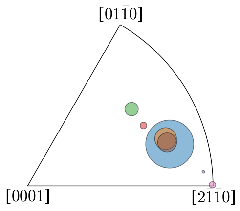
Inspect rotation axes of clusters (in the axis-angle representation) in an inverse pole figure

cluster_sizes_scaled = 5000 * cluster_sizes / cluster_sizes.max()
fig, ax = plt.subplots(
    figsize=(5, 5), subplot_kw=dict(projection="ipf", symmetry=D6)
)
ax.scatter(
    cluster_means.axis, c=colors, s=cluster_sizes_scaled, alpha=0.5, ec="k"
)

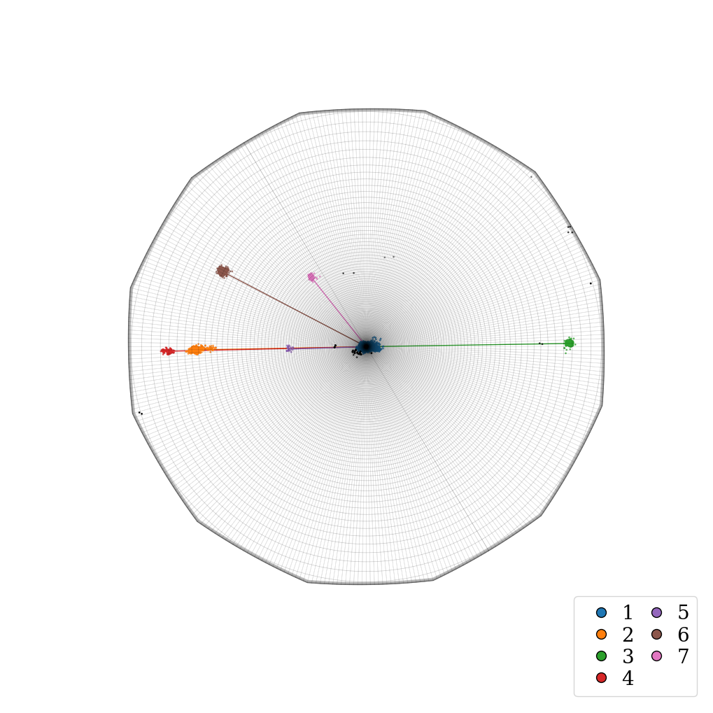
Plot a top view of the recentered orientation clusters within the fundamental zone for the D6 (622) point group symmetry of Ti. The mean orientation of the largest parent grain is taken as the reference orientation.

wireframe_kwargs = dict(
    color="black", linewidth=0.5, alpha=0.1, rcount=181, ccount=361
)
fig = ori_recentered.scatter(
    projection="axangle",
    wireframe_kwargs=wireframe_kwargs,
    c=labels_rgb.reshape(-1, 3),
    s=1,
    return_figure=True,
)
ax = fig.axes[0]
ax.view_init(elev=90, azim=-30)
ax.add_collection3d(Line3DCollection(lines, colors=colors))

handle_kwds = dict(marker="o", color="none", markersize=10)
handles = []
for i in range(n_clusters):
    line = Line2D(
        [0], [0], label=i + 1, markerfacecolor=colors[i], **handle_kwds
    )
    handles.append(line)
ax.legend(
    handles=handles,
    loc="lower right",
    ncol=2,
    numpoints=1,
    labelspacing=0.15,
    columnspacing=0.15,
    handletextpad=0.05,
);

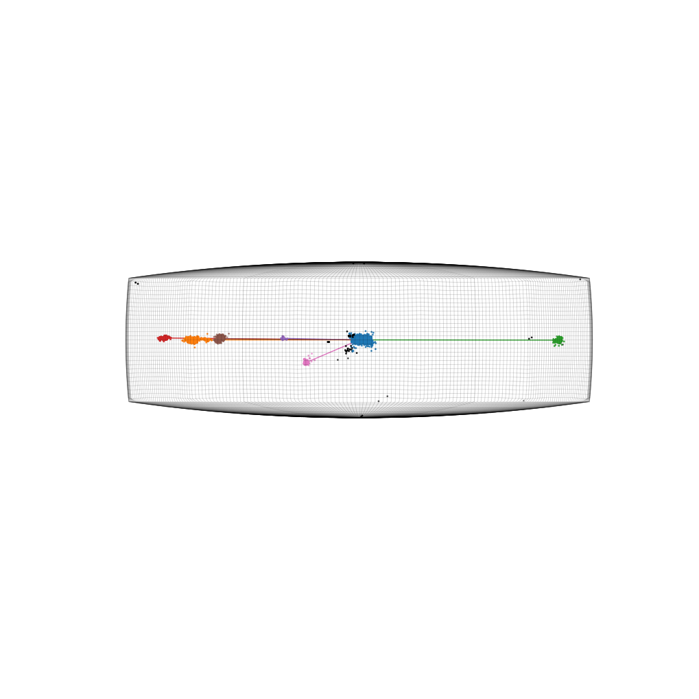
Plot side view of orientation clusters

fig2 = ori_recentered.scatter(
    return_figure=True,
    wireframe_kwargs=wireframe_kwargs,
    c=labels_rgb.reshape(-1, 3),
    s=1,
)
ax2 = fig2.axes[0]
ax2.add_collection3d(Line3DCollection(lines, colors=colors))
ax2.view_init(elev=0, azim=-30)

Plot map indicating spatial locations associated with each cluster

fig3, ax3 = plt.subplots(figsize=(15, 10))
ax3.imshow(labels_rgb)
ax3.axis("off");