This page was generated from doc/tutorials/inverse_pole_figures.ipynb. Interactive online version: .

Inverse pole figures

In this tutorial we will express in which crystal direction \(\mathbf{t} = \left<uvw\right>\) any sample direction \(\mathbf{v} = (x, y, z)\), or any Vector3d, is parallel to. Formally, this so-called inverse pole figure (IPF) shows the directional distribution of a set of reference vectors in terms of a fixed crystallographic frame [Nolze, 2015]. By assigning a unique colour to each crystal direction in a symmetry’s fundamental sector (the IPF), we can colour orientations [Nolze and Hielscher, 2016].

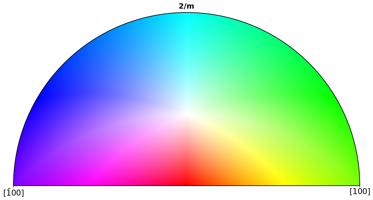
While orix has descriptions for all 32 crystallographic point groups \(S\), so far only the fundamental sectors of the eleven Laue group symmetries have been defined. Thus, the Laue class (in the left and center column in the table below) of the point groups (center and right column) will be used when plotting the IPF and colouring orientations.

Schoenflies	Laue	Non-centrosymmetric
\(Ci\)	\(\bar{1}\)	\(1\)
\(C2h\)	\(2/m\)	\(2\), \(m\)
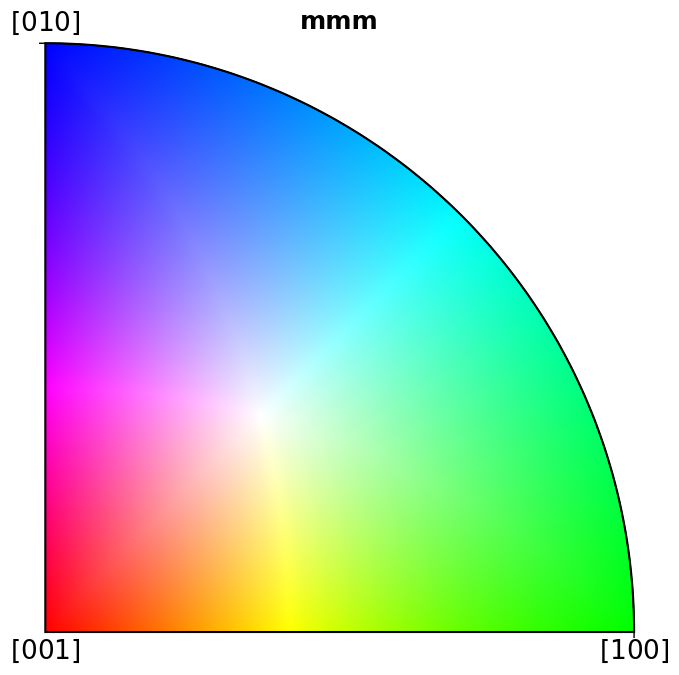
\(D2h\)	\(mmm\)	\(222\), \(2mm\)
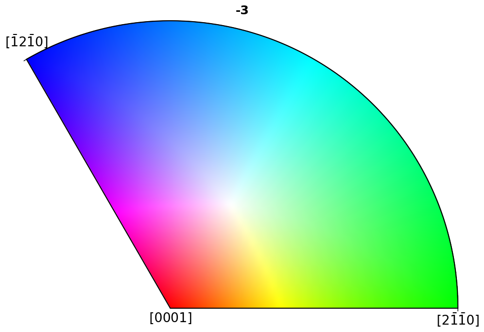
\(S6\)	\(\bar{3}\)	\(3\)
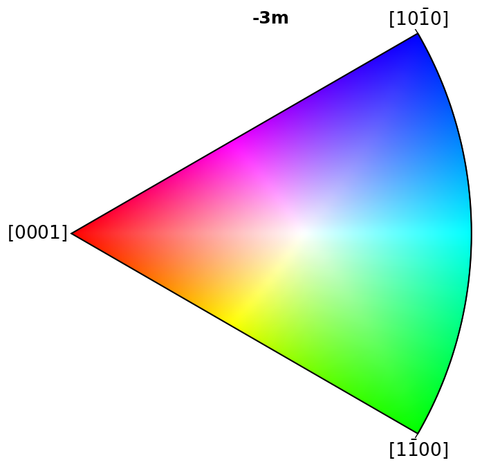
\(D3d\)	\(\bar{3}m\)	\(32\), \(3m\)
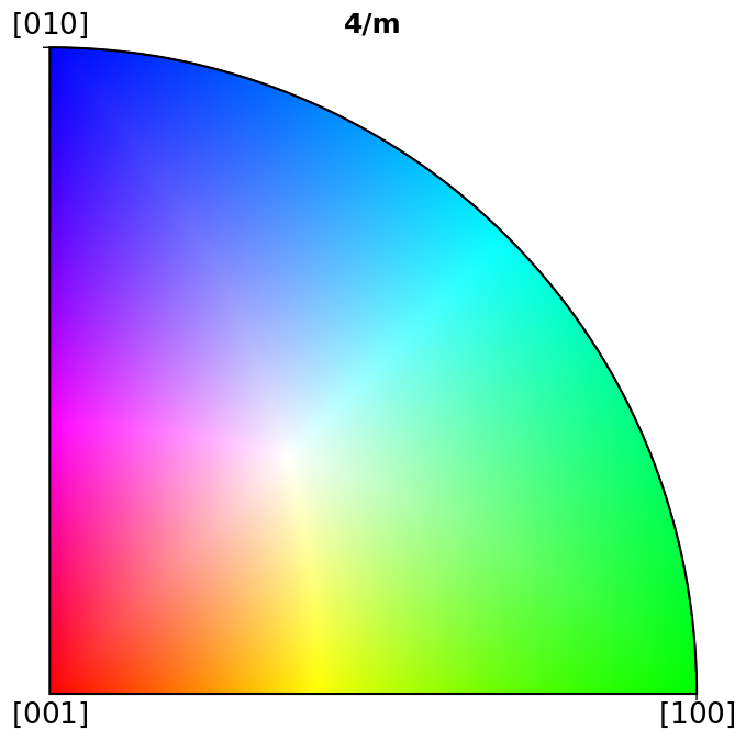
\(C4h\)	\(4/m\)	\(4\), \(\bar{4}\)
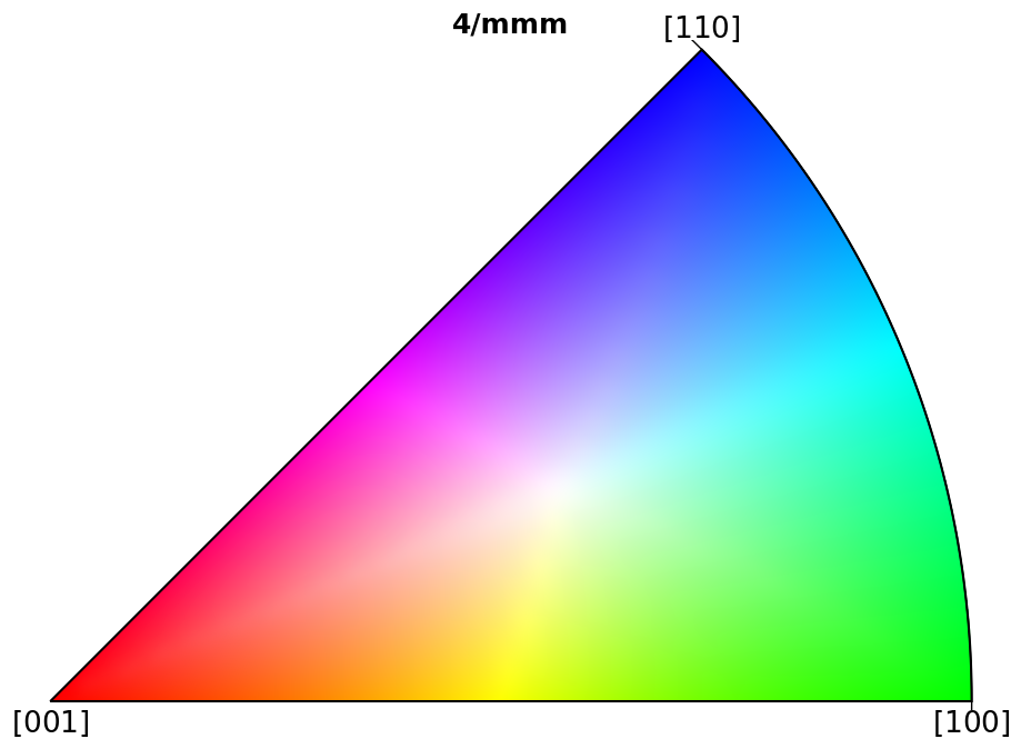
\(D4h\)	\(4/mmm\)	\(422\), \(\bar{4}2m\), \(4mm\)
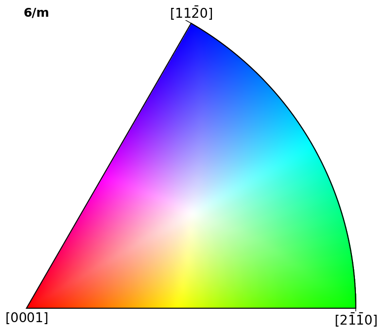
\(C6h\)	\(6/m\)	\(6\), \(\bar{6}\)
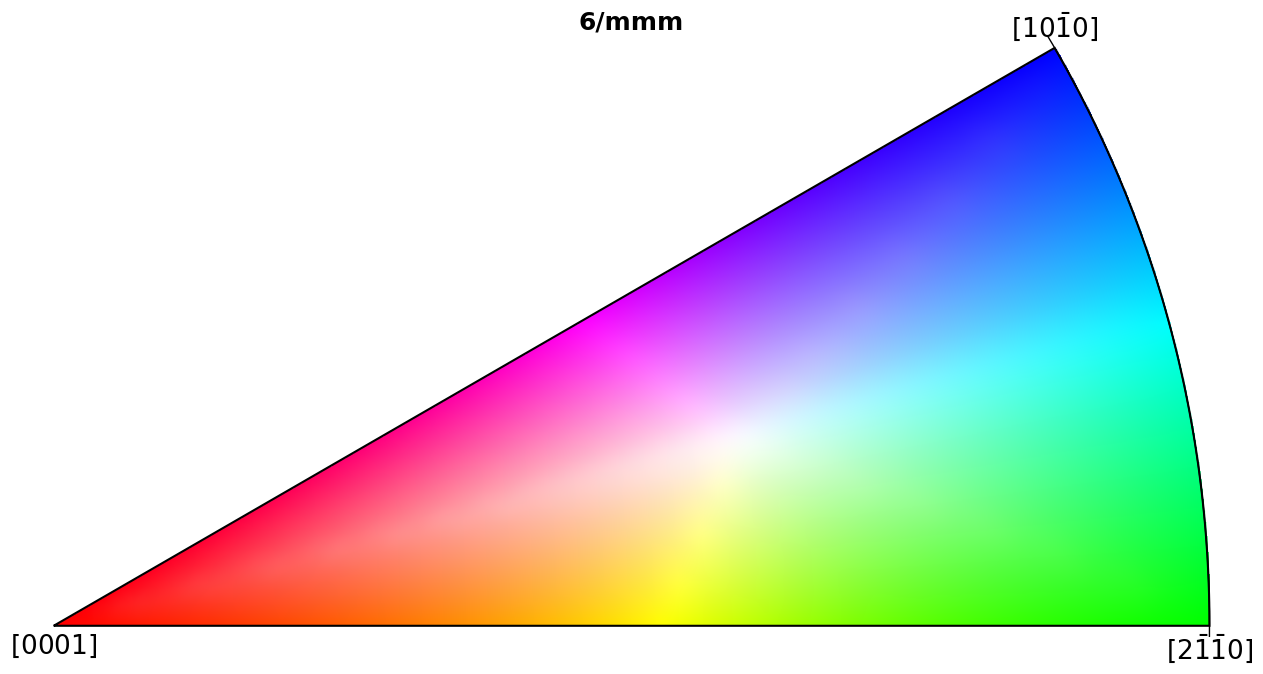
\(D6h\)	\(6/mmm\)	\(622\), \(\bar{6}2m\), \(6mmm\)
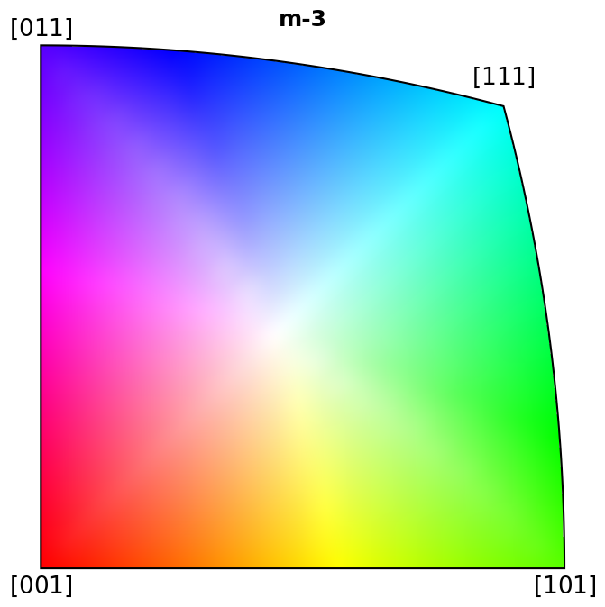
\(Th\)	\(m\bar{3}\)	\(23\)
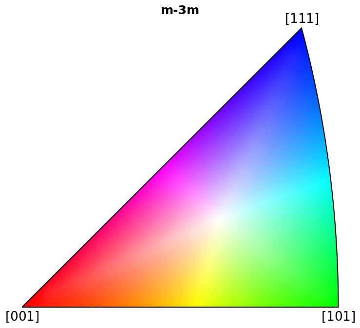
\(Oh\)	\(m\bar{3}m\)	\(432\), \(\bar{4}3m\)

Only the colour keys used in EDAX TSL OIM Analysis are supported, via the IPFColorKeyTSL.

The IPF functionality in the excellent software MTEX and the two above referenced works have been the basis for the IPF functionality in orix.

%matplotlib inline

import matplotlib.pyplot as plt
import numpy as np

from orix import plot, sampling
from orix.crystal_map import Phase
from orix.quaternion import Orientation, symmetry
from orix.vector import Vector3d


# We'll want our plots to look a bit larger than the default size
new_params = {
    "figure.facecolor": "w",
    "figure.figsize": (20, 7),
    "lines.markersize": 10,
    "font.size": 15,
    "axes.grid": True,
}
plt.rcParams.update(new_params)

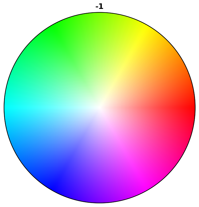
Minimal example of plotting the IPF colour key

plot.IPFColorKeyTSL(symmetry.D3d).plot()

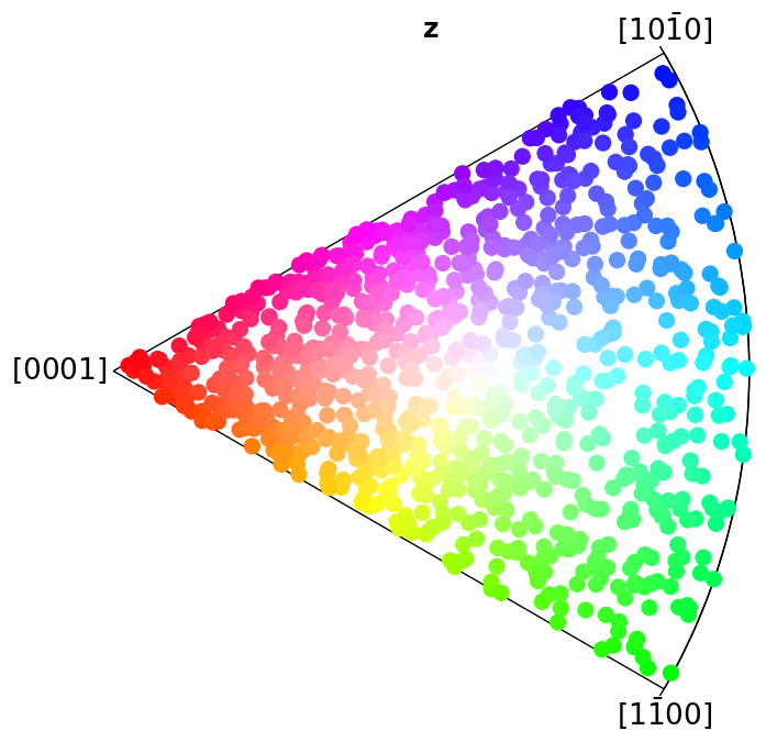
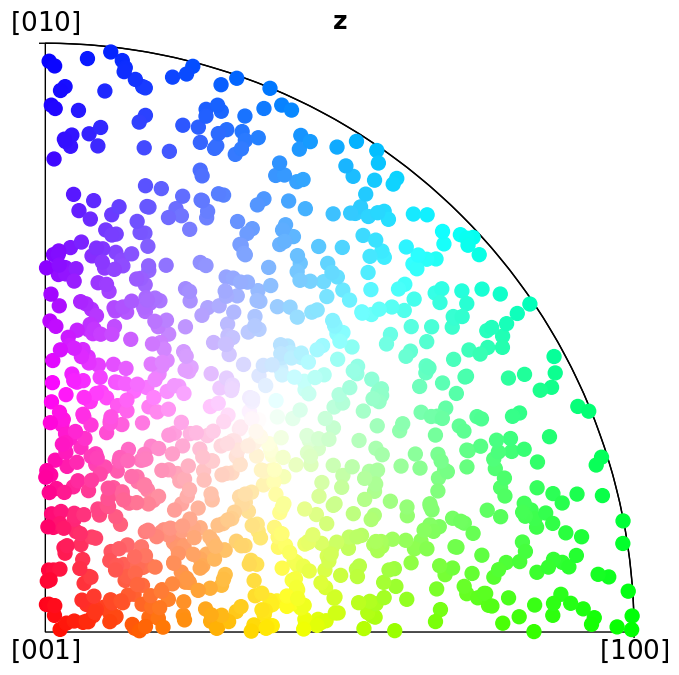
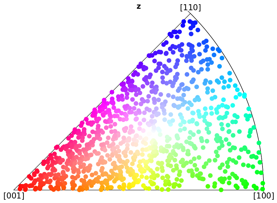
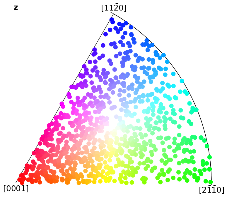
Plot colour keys

Here we plot the colour keys for the eleven Laue groups. An example demonstrating how an IPF color key can be added to a custom plot is shown in the Crystal map tutorial.

pg_laue = [
    symmetry.Ci,
    symmetry.C2h,
    symmetry.D2h,
    symmetry.S6,
    symmetry.D3d,
    symmetry.C4h,
    symmetry.D4h,
    symmetry.C6h,
    symmetry.D6h,
    symmetry.Th,
    symmetry.Oh,
]

for pg in pg_laue:
    ipfkey = plot.IPFColorKeyTSL(pg)
    ipfkey.plot()

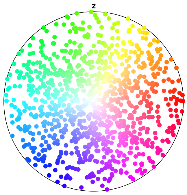
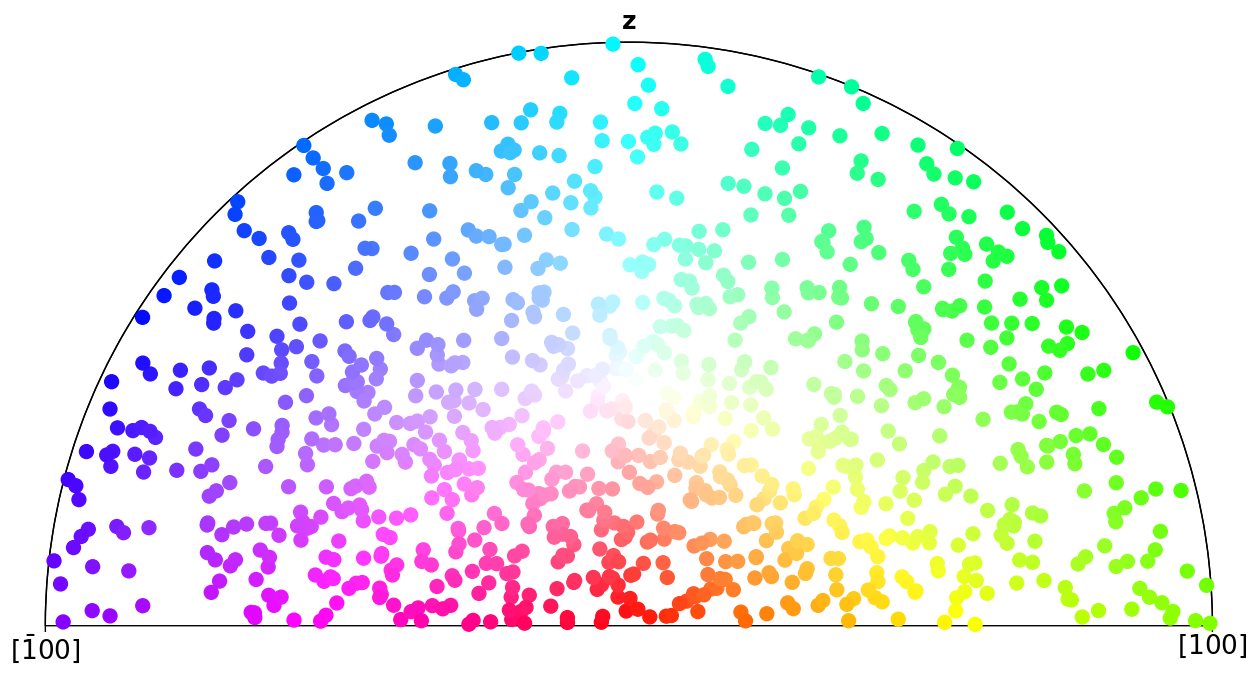
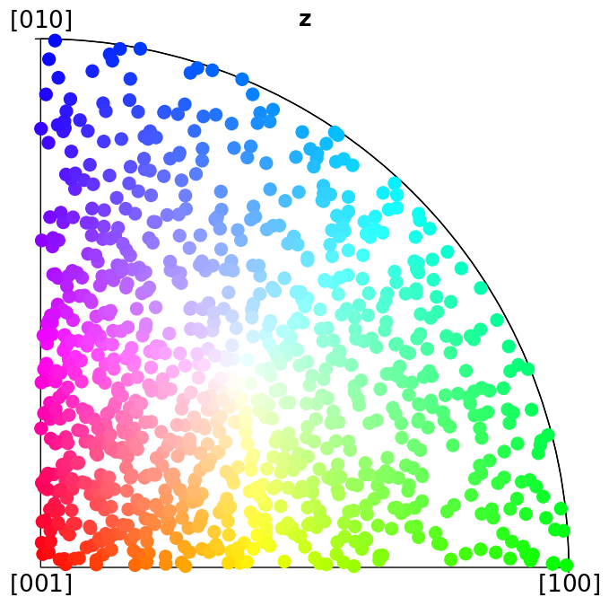
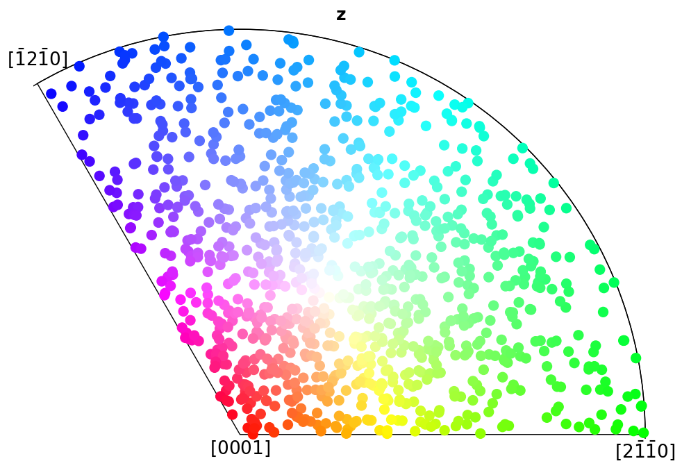
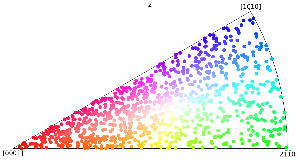
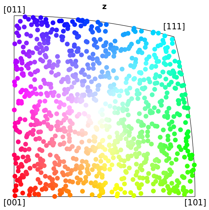
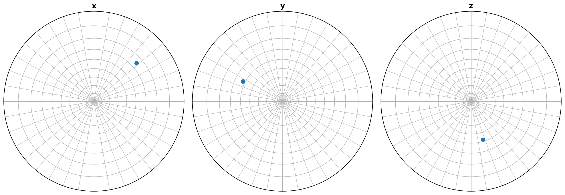
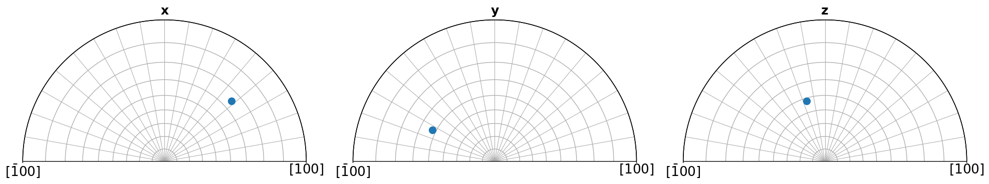
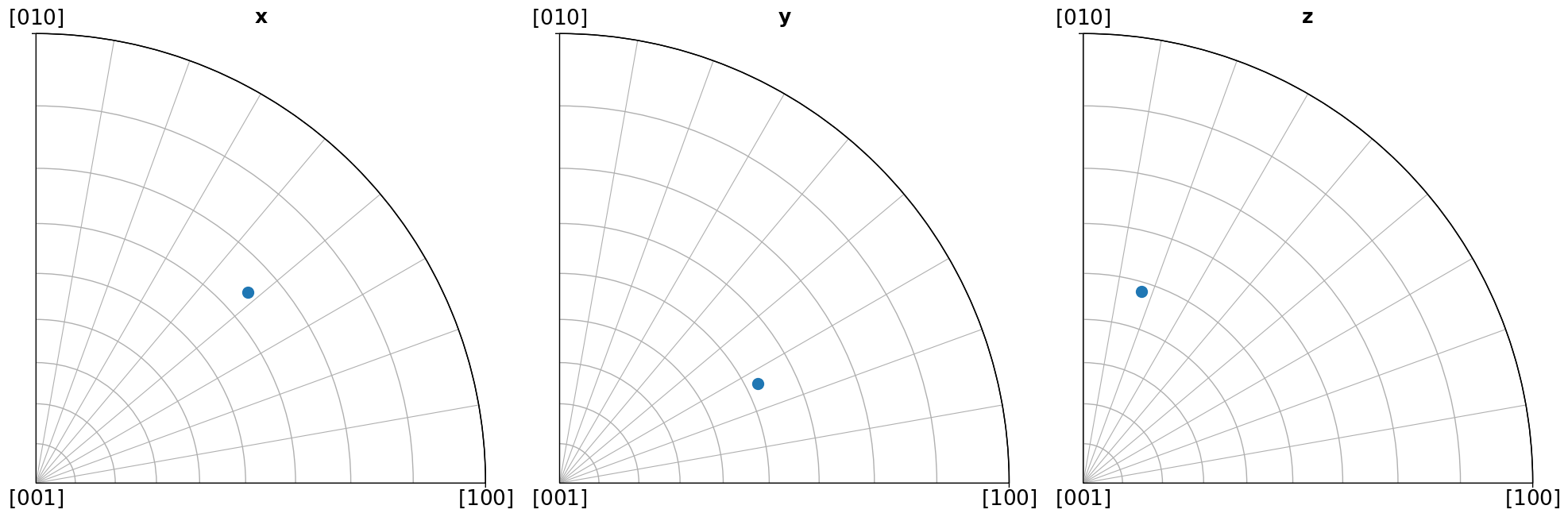
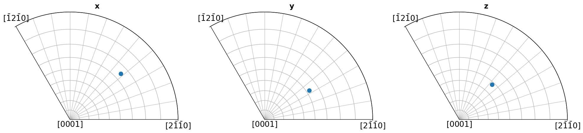
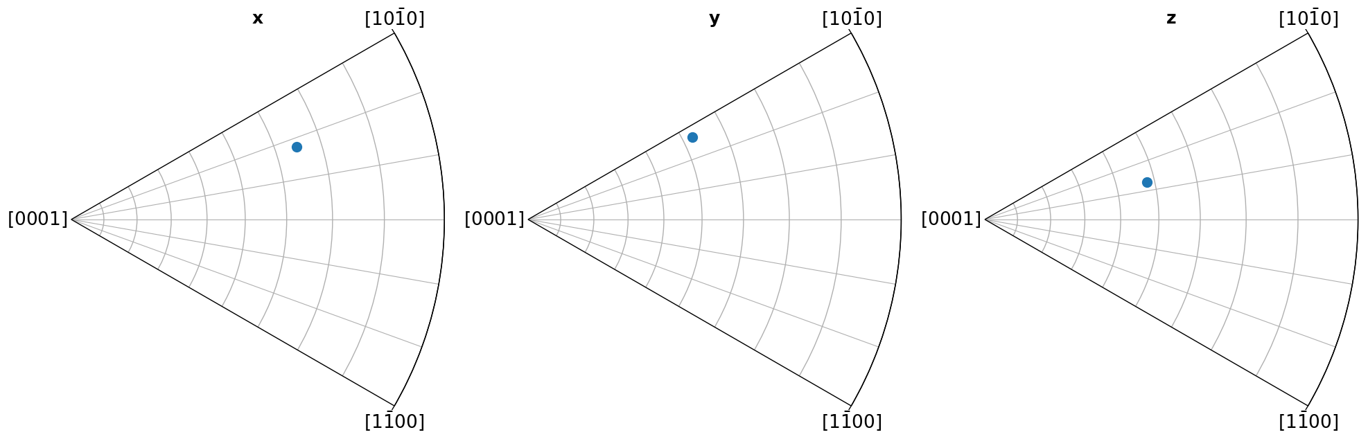
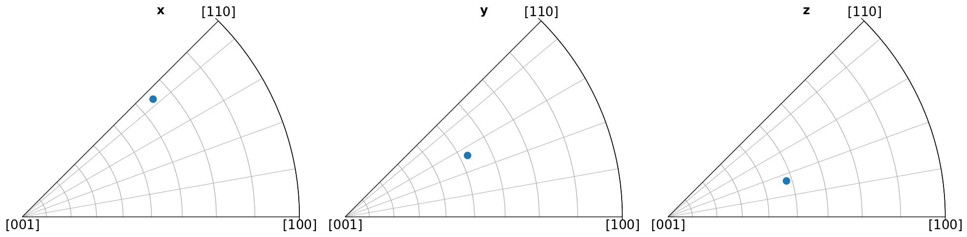
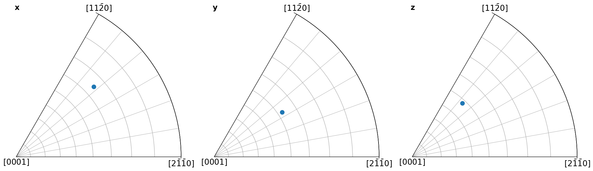
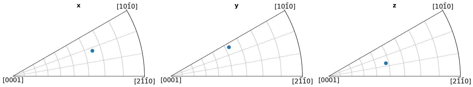
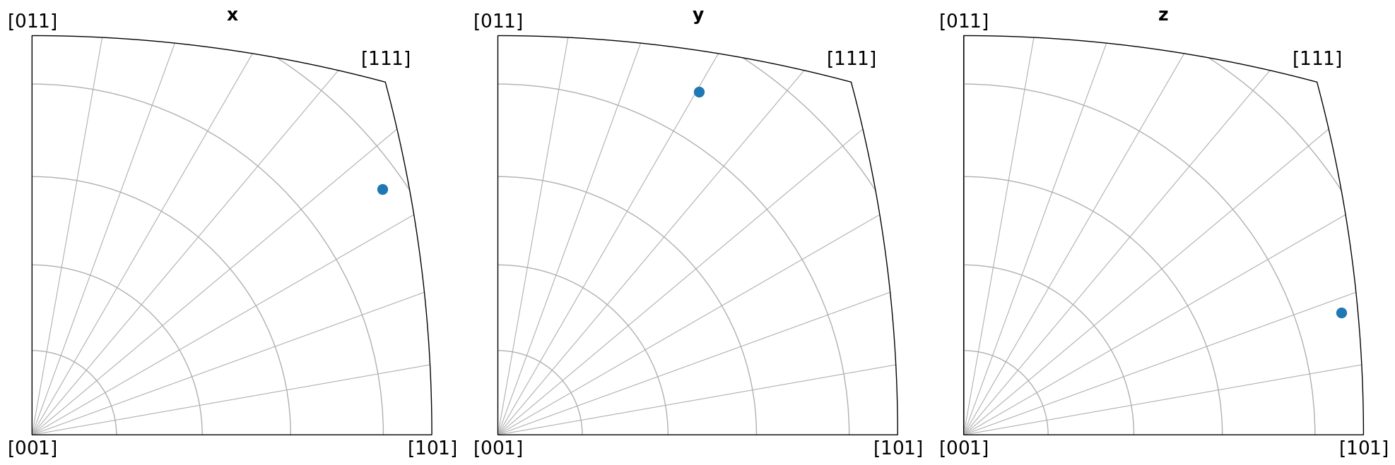
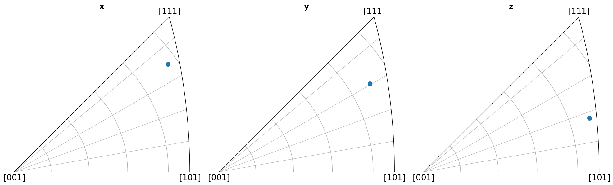
Scatter plot

Here we show which crystal direction \(\left<uvw\right>\) the sample reference frame directions \((x, y, Z)\) point in. We can turn off the grid by updating the Matplotlib parameters with plt.rcParams["axes.grid"] = False, or passing grid=False to Orientation.scatter(), which we use to plot the IPFs.

v = Vector3d([[1, 0, 0], [0, 1, 0], [0, 0, 1]])
kwargs = {"projection": "ipf", "direction": v}

for S in pg_laue:
    O = Orientation.from_euler([325, 48, 163], S, degrees=True)
    O.scatter(**kwargs)

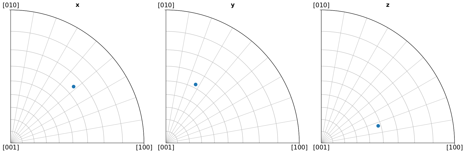
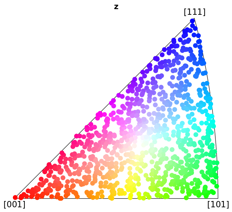
Coloring orientations

Here we show how to obtain an RGB colour for each crystal orientation given a sample direction, using IPFColorKeyTSL.orientation2color. We then plot them in the IPF. Note that we could instead plot them in a map, say when the orientations come from a crystallographic mapping experiment. See the crystal map tutorial for an example.

plt.rcParams["axes.grid"] = False

O2 = Orientation.random(1000)
for S in pg_laue:
    ipfkey = plot.IPFColorKeyTSL(S)
    O2.symmetry = ipfkey.symmetry
    rgb_z = ipfkey.orientation2color(O2)
    O2.scatter("ipf", c=rgb_z, direction=ipfkey.direction)