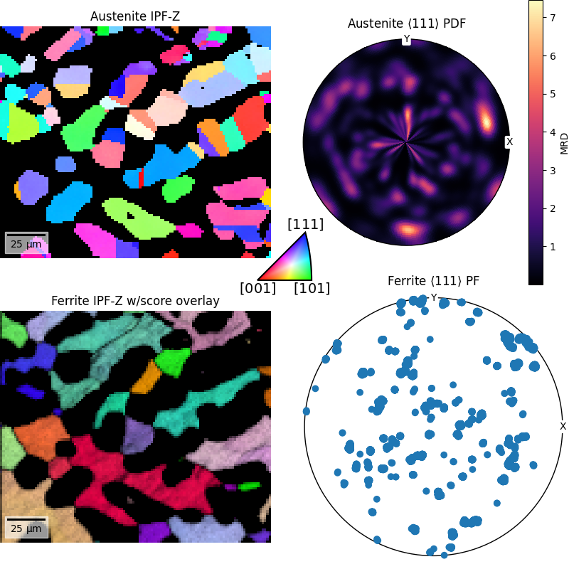
Subplots

This example shows how to place different plots in the same figure using orix’ various plot types, which extend Matplotlib’s plot types.

By first creating a blank figure and then using add_subplot() to add various orix plot types, we build up a figure with two rows and two columns showing separate orientation maps (IPF-Z maps) of two phases, a pole density function (PDF) and a discrete pole figure (PF).

Out:

Phase   Orientations       Name  Space group  Point group  Proper point group       Color
    1   5657 (48.4%)  austenite         None          432                 432    tab:blue
    2   6043 (51.6%)    ferrite         None          432                 432  tab:orange
Properties: iq, dp
Scan unit: um

import matplotlib.pyplot as plt

from orix import data, plot
from orix.vector import Miller

xmap = data.sdss_ferrite_austenite(allow_download=True)
print(xmap)

pg_laue = xmap.phases[1].point_group.laue
o_au = xmap["austenite"].orientations
o_fe = xmap["ferrite"].orientations

# Orientation colors
ipf_key = plot.IPFColorKeyTSL(pg_laue)
rgb_au = ipf_key.orientation2color(o_au)
rgb_fe = ipf_key.orientation2color(o_fe)

# Austenite <111> poles in the sample reference frame
uvw_au = Miller(uvw=[1, 1, 1], phase=xmap.phases["austenite"]).symmetrise(unique=True)
uvw_au_all = (~o_au).outer(uvw_au)

# Ferrite <111> poles in the sample reference frame
uvw_fe = Miller(uvw=[1, 1, 1], phase=xmap.phases["ferrite"]).symmetrise(unique=True)
uvw_fe_all = (~o_fe).outer(uvw_fe)

# Create figure
fig = plt.figure(figsize=(8, 8))

ax0 = fig.add_subplot(221, projection="plot_map")
ax0.plot_map(xmap["austenite"], rgb_au)
ax0.set_title("Austenite IPF-Z")
ax0.remove_padding()

ax1 = fig.add_subplot(222, projection="stereographic")
ax1.pole_density_function(uvw_au_all)
ax1.set_labels("X", "Y", None)
ax1.set_title(r"Austenite $\left<111\right>$ PDF")

ax2 = fig.add_subplot(223, projection="plot_map")
ax2.plot_map(xmap["ferrite"], rgb_fe)
ax2.add_overlay(xmap["ferrite"], xmap["ferrite"].dp)
ax2.set_title("Ferrite IPF-Z w/score overlay")
ax2.remove_padding()

ax3 = fig.add_subplot(224, projection="stereographic")
ax3.scatter(uvw_fe_all)
ax3.set_labels("X", "Y", None)
ax3.set_title(r"Ferrite $\left<111\right>$ PF")

# Place the IPF color key carefully in the center over the other figures
ax_ckey = fig.add_axes(
    [0.45, 0.5, 0.1, 0.1], projection="ipf", symmetry=pg_laue, zorder=2
)
ax_ckey.plot_ipf_color_key()
ax_ckey.set_title(None)
ax_ckey.patch.set_facecolor("None")

fig.subplots_adjust(hspace=0, wspace=0.1)

Estimated memory usage: 29 MB