Visualizing orientations

This example shows how to visualize orientations using various projections. Visualizing orientations requires defining some projection between orientation space and Euclidean space, which will by necessity introduce distortion. This problem is similar to how any 2D map of Earth’s surface will always have a spatially-dependent scalebar.

Three 3D projections representing orientations as axis-angle pairs are available. Additionally, a 2D projection, given a sample direction, in the stereographic projection is available.

The three axis-angle projections, sometimes called Neo-Eulerian projections, describe a rotation by a twist \(\omega\) around an axis \(\hat{\mathbf{n}}\). The \((x, y, z)\) coordinates of the rotation’s projection are the \((v_x, v_y, v_z)\) coordinates of a unit vector describing \(\hat{\mathbf{n}}\), scaled by a function of \(\omega\). The scaling options are:

• axis-angle pair: a linear projection \(\omega \cdot \hat{\mathbf{n}}\). Available in AxAnglePlot.

• Rodrigues vector: a rectilinear projection \(\tan\omega/2 \cdot \hat{\mathbf{n}}\), where rotations sharing a common rotation axis are linearly aligned. Available in RodriguesPlot.

• homochoric vector: an equal-volume projection \(0.75(\omega-\sin\omega)^{\frac{1}{3}} \cdot \hat{\mathbf{n}}\), where a cube anywhere inside takes up an identical solid angle in rotation space. Available in HomochoricPlot.

Note that this list is not exhaustive and that the descriptions are simplified. For a deeper dive into the advantages and disadvantages of these projections, as well as enlightening comparisons of their warping of orientation space, refer to the [Krakow et al., 2017].

The 2D projection in the stereographic projection is the so-called inverse pole figure (IPF). This shows which crystal direction \(\mathbf{t} = \left<uvw\right>\) a given sample direction \(\mathbf{v} = (x, y, z)\) is parallel to. The crystal direction is given in the fundamental sector of an orientations point group and projected down to the equatorial plane using the stereographic projection \((X, Y) = (v_x / (1 - v_z), v_y / (1 - v_z))\). This is computationally efficient and translates well to print publication. However, the projection loses orientation information perpendicular to the sample direction plotted, a bit like a 2D X-ray of a skeleton.

The projections are implemented by subclassing Matplotlib’s matplotlib.axes.Axes and mpl_toolkits.mplot3d.axes3d.Axes3D.

import matplotlib.pyplot as plt
import numpy as np

from orix.plot import IPFColorKeyTSL, register_projections
from orix.quaternion import Orientation, OrientationRegion
from orix.quaternion.symmetry import D3

register_projections()  # Register our custom Matplotlib projections
np.random.seed(2319)  # Create reproducible random data

n = 30
ori = Orientation.random(n, symmetry=D3)

# Create an orientation-dependent colormap for more informative plots
color_key = IPFColorKeyTSL(D3)
rgb = color_key.orientation2color(ori)

Orientation plots can be made in one of two ways. The first and simplest is via scatter().

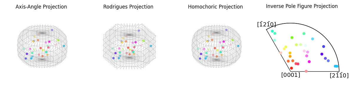
fig = plt.figure(figsize=(12, 3), layout="tight")
ori.scatter(c=rgb, position=141, projection="axangle", figure=fig)
fig.axes[0].set_title("Axis-Angle Projection")
ori.scatter(c=rgb, position=142, projection="rodrigues", figure=fig)
fig.axes[1].set_title("Rodrigues Projection")
ori.scatter(c=rgb, position=143, projection="homochoric", figure=fig)
fig.axes[2].set_title("Homochoric Projection")
ori.scatter(c=rgb, position=144, projection="ipf", figure=fig)
_ = fig.axes[3].set_title("Inverse Pole Figure Projection \n\n")

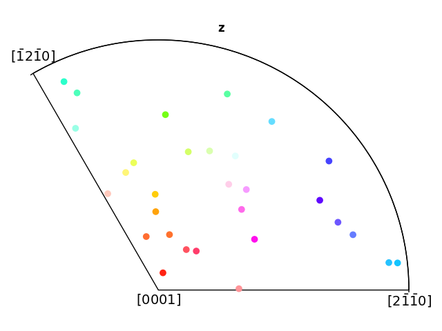
This can also be used to create standalone figures

ori.scatter(c=rgb, projection="ipf")

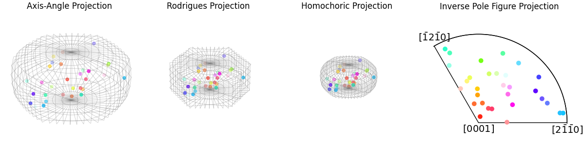
The second method is by setting the projections when defining the Matplotlib axes. This can require more tinkering since the plots are not auto-formatted like above, but it allows for more customization as well as the plotting of multiple datasets on a single plot

Additionally, for these plots, we will set the scaling equivalent in order to better illustrate the differences in the scales of the Neo-Eulerian plotting methods.

fig = plt.figure(figsize=(12, 3), layout="constrained")
ax_ax = fig.add_subplot(141, projection="axangle")
ax_rod = fig.add_subplot(142, projection="rodrigues")
ax_hom = fig.add_subplot(143, projection="homochoric")
ax_ipf = fig.add_subplot(144, projection="ipf", symmetry=D3)

ax_ipf.scatter(ori, c=rgb)

ax_ax.set_title("Axis-Angle Projection")
ax_rod.set_title("Rodrigues Projection")
ax_hom.set_title("Homochoric Projection")
ax_ipf.set_title("Inverse Pole Figure Projection \n\n")

fundamental_zone = OrientationRegion.from_symmetry(ori.symmetry)

for ax in [ax_ax, ax_rod, ax_hom]:
    ax.plot_wireframe(fundamental_zone)
    ax.set_proj_type = "ortho"
    ax.axis("off")
    ax.set(xlim=(-1.2, 1.2), ylim=(-1.2, 1.2), zlim=(-1.2, 1.2))
    ax.scatter(ori, c=rgb)

Estimated memory usage: 553 MB