Crystal reference frame

This exampe shows how the crystal and sample reference frames are aligned for a Phase.

from diffpy.structure import Lattice, Structure
import matplotlib.pyplot as plt
import numpy as np

from orix.crystal_map import Phase
from orix.quaternion import Rotation
from orix.vector import Miller

plt.rcParams.update(
    {
        "figure.figsize": (10, 5),
        "font.size": 20,
        "axes.grid": True,
        "lines.markersize": 10,
        "lines.linewidth": 3,
    }
)

Alignment and the structure matrix

The direct Bravais lattice is characterized by basis vectors \((\mathbf{a}, \mathbf{b}, \mathbf{c})\) with unit cell edge lengths :math:(a, b, c) and angles \((\alpha, \beta, \gamma)\). The reciprocal lattice has basis vectors given by

\[\mathbf{a^*} = \frac{\mathbf{b} \times \mathbf{c}}{\mathbf{a} \cdot (\mathbf{b} \times \mathbf{c})},\:\: \mathbf{b^*} = \frac{\mathbf{c} \times \mathbf{a}}{\mathbf{a} \cdot (\mathbf{b} \times \mathbf{c})},\:\: \mathbf{c^*} = \frac{\mathbf{a} \times \mathbf{b}}{\mathbf{a} \cdot (\mathbf{b} \times \mathbf{c})},\]

with reciprocal lattice parameters \((a^*, b^*, c^*)\) and angles \((\alpha^*, \beta^*, \gamma^*)\).

Using these two crystallographic lattices, we can define a standard Cartesian (orthonormal) reference frame by the unit vectors \((\mathbf{e_1}, \mathbf{e_2}, \mathbf{e_3})\). In principle, the direct lattice reference frame can be oriented arbitrarily in the Cartesian reference frame. In orix we have chosen

\[\mathbf{e_1} ||\: \frac{\mathbf{a}}{a},\:\: \mathbf{e_2} ||\: \mathbf{e_3} \times \mathbf{e_1},\:\: \mathbf{e_3} ||\: \frac{\mathbf{c^*}}{c^*}.\]

This alignment is used for example in [Rowenhorst et al., 2015] and [De Graef, 2003], the latter which was the basis for the EMsoft Fortran suite of programs. Another common option is \(\mathbf{e_1} || \mathbf{a^*}/a^*, \mathbf{e_2} || \mathbf{e_3} \times \mathbf{e_1}, \mathbf{e_3} || \mathbf{c}/c\), which is used for example in [Britton et al., 2016] and the diffpy.structure Python package, which we’ll come back to.

In calculations, it is useful to describe the transformation of the Cartesian unit row vectors to the coordinates of the direct lattice vectors by the structure row matrix \(\mathbf{A}\) (also called the crystal base). Given the chosen alignment of basis vectors with the Cartesian reference frame, \(\mathbf{A}\) is defined as

\[\begin{split}\begin{equation} \mathbf{A} = \begin{pmatrix} a & 0 & 0\\ b\cos\gamma & b\sin\gamma & 0\\ c\cos\beta & -c\frac{(\cos\beta\cos\gamma - \cos\alpha)}{\sin\gamma} & \frac{\mathrm{V}}{ab\sin\gamma} \end{pmatrix}, \end{equation}\end{split}\]

where \(V\) is the volume of the unit cell.

In orix, we use the Lattice class to keep track of these properties internally.

Let’s create an hexagonal crystal with lattice parameters \((a, b, c)\) = (1.4, 1.4, 1.7) nm and \((\alpha, \beta, \gamma) = (90^{\circ}, 90^{\circ}, 120^{\circ})\)

lat = Lattice(1.4, 1.4, 1.7, 90, 90, 120)
print(lat)

Lattice(a=1.4, b=1.4, c=1.7, alpha=90, beta=90, gamma=120)

diffpy.structure stores the structure matrix in the base property

print(lat.base)

[[ 1.21243557 -0.7         0.        ]
 [ 0.          1.4         0.        ]
 [ 0.          0.          1.7       ]]

We see that diffpy.structure does not use the orix alignment mentioned above, since \(\mathbf{e1} \nparallel \mathbf{a} / a\). Instead, we see that \(\mathbf{e3} \parallel \mathbf{c} / c\), which is in line with the alternative alignment mentioned above.

Thus, the alignment is updated internally whenever a Phase is created, a class which brings together this crystal lattice and a point group Symmetry S

structure_hex = Structure(lattice=lat)
phase_hex = Phase(point_group="6/mmm", structure=structure_hex)
print(phase_hex.structure.lattice.base)

[[ 1.4         0.          0.        ]
 [-0.7         1.21243557  0.        ]
 [ 0.          0.          1.7       ]]

Caution

Using another alignment than the one described above has undefined behaviour in orix. Therefore, it is important that the structure matrix of a phase is not changed.

Note

The lattice is included in a Structure because the latter class brings together a lattice and Atom s, which is useful when simulating diffraction.

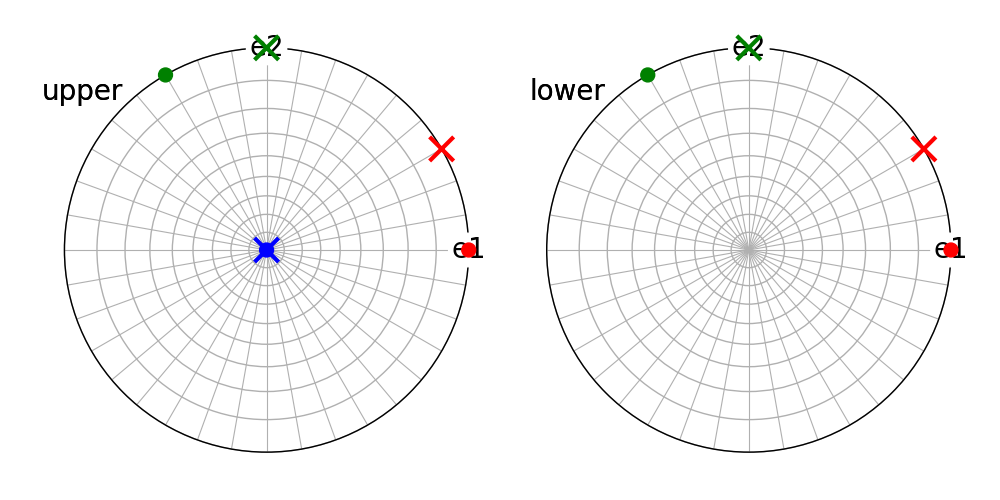
We can visualize the alignment of the direct and reciprocal lattice basis vectors with the Cartesian reference frame using the stereographic projection

t_hex = Miller(uvw=[[1, 0, 0], [0, 1, 0], [0, 0, 1]], phase=phase_hex)
g_hex = Miller(hkl=[[1, 0, 0], [0, 1, 0], [0, 0, 1]], phase=phase_hex)

fig = t_hex.scatter(
    c=["r", "g", "b"],
    marker="o",
    return_figure=True,
    axes_labels=["e1", "e2"],
    hemisphere="both",
)
g_hex.scatter(c=["r", "g", "b"], marker="x", s=300, figure=fig)

Alignment of symmetry operations

To see which crystallographic axes the point group symmetry operations rotate about, we can add symmetry operations to the figure and show it again

R = Rotation.from_axes_angles([0, 1, 0], -65, degrees=True)
phase_hex.point_group.plot(figure=fig, orientation=R)

fig

<Figure size 1000x500 with 2 Axes>

Converting crystal vectors

The reference frame of the stereographic projection above is the Cartesian reference frame \((\mathbf{e_1}, \mathbf{e_2}, \mathbf{e_3})\). The Cartesian coordinates \((\mathbf{x}, \mathbf{y}, \mathbf{z})\) of \((\mathbf{a}, \mathbf{b}, \mathbf{c})\) and \((\mathbf{a^*}, \mathbf{b^*}, \mathbf{c^*})\) were found using \(\mathbf{A}\) in the following conversions

\[\begin{split}\begin{align} (x, y, z) &= [uvw] \cdot \mathbf{A},\\ (x, y, z) &= (hkl) \cdot (\mathbf{A}^{-1})^T. \end{align}\end{split}\]

Let’s compute the internal conversions directly and check for equality

A = phase_hex.structure.lattice.base
v1 = np.dot(t_hex.uvw, A)
print(np.allclose(t_hex.data, v1))

v2 = np.dot(g_hex.hkl, np.linalg.inv(A).T)
print(np.allclose(g_hex.data, v2.data))

plt.show()

True
True

Estimated memory usage: 549 MB