Clustering misorientations#
In this tutorial we will cluster Ti crystal misorientations using data obtained from a highly deformed specimen, using EBSD, as presented in [Johnstone et al., 2020]. The data can be downloaded to your local cache via the orix.data module.
Import orix classes and various dependencies
[1]:
# Exchange "inline" for "notebook" (or "qt5" from pyqt) for interactive plotting
%matplotlib inline

from matplotlib.colors import to_rgb
from matplotlib.lines import Line2D
import matplotlib.pyplot as plt
import numpy as np
from skimage.color import label2rgb
from sklearn.cluster import DBSCAN

from orix.plot import register_projections, IPFColorKeyTSL
from orix import data
from orix.quaternion import Misorientation, Rotation
from orix.vector import Vector3d

plt.rcParams.update({"font.size": 20, "figure.figsize": (10, 10)})

register_projections()
Import data#
Load Ti orientations with the point group symmetry 622 (D6). We have to explicitly allow downloading from an external source.
[2]:
ori = data.ti_orientations(allow_download=True)
ori
/home/docs/checkouts/readthedocs.org/user_builds/orix/conda/latest/lib/python3.14/site-packages/tqdm/auto.py:21: TqdmWarning: IProgress not found. Please update jupyter and ipywidgets. See https://ipywidgets.readthedocs.io/en/stable/user_install.html
  from .autonotebook import tqdm as notebook_tqdm
[2]:
Orientation (193167,) 622
[[ 0.3027  0.0869 -0.5083  0.8015]
 [ 0.3088  0.0868 -0.5016  0.8034]
 [ 0.3057  0.0818 -0.4995  0.8065]
 ...
 [ 0.4925 -0.1633 -0.668   0.5334]
 [ 0.4946 -0.1592 -0.6696  0.5307]
 [ 0.4946 -0.1592 -0.6696  0.5307]]
Extract the symmetry
[3]:
sym = ori.symmetry
Reshape the orientation mapping data to the correct spatial dimension for the scan and select a subset of the orientations with a suitable size for this demonstration (bottom left corner)
[4]:
ori = ori.reshape(381, 507)
ori = ori[-100:, :200]
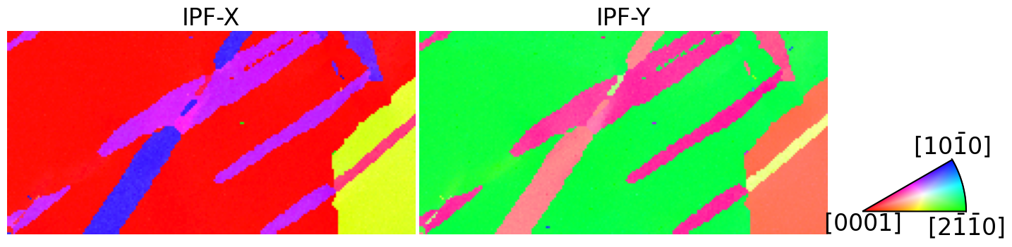
Plot orientation maps
[5]:
ckey = IPFColorKeyTSL(sym)

directions = [(1, 0, 0), (0, 1, 0)]
titles = ["X", "Y"]

fig, axes = plt.subplots(ncols=2, figsize=(15, 10))
for i, ax in enumerate(axes):
    ckey.direction = Vector3d(directions[i])
    ax.imshow(ckey.orientation2color(ori))
    ax.set_title(f"IPF-{titles[i]}")
    ax.axis("off")

# Add color key
ax_ipfkey = fig.add_axes(
    [0.932, 0.37, 0.1, 0.1],  # (Left, bottom, width, height)
    projection="ipf",
    symmetry=ori.symmetry.laue,
)
ax_ipfkey.plot_ipf_color_key()
ax_ipfkey.set_title("")
fig.subplots_adjust(wspace=0.01)
Map the orientations into the Rodrigues fundamental zone (find symmetrically equivalent orientations with the smallest angle of rotation) of 622
[6]:
ori = ori.reduce()
Compute misorientations \(m_{AB} = g_B \cdot g_A^{-1}\) (in the horizontal direction)
[7]:
mori_all = Misorientation(ori[:, :-1] * ~ori[:, 1:], symmetry=(sym, sym))
Keep only misorientations with a disorientation angle higher than 7\(^{\circ}\), assumed to represent grain boundaries
[8]:
boundary_mask = mori_all.angle > np.deg2rad(7)
mori = mori_all[boundary_mask]
Map the misorientations into the fundamental zone of 622-622
[9]:
mori = mori.reduce()
Compute distance matrix#
[10]:
D = mori.get_distance_matrix(lazy=False)
Clustering#
Apply mask to remove small misorientations associated with grain orientation spread
[11]:
small_mask = mori.angle < np.deg2rad(7)
D = D[~small_mask][:, ~small_mask]
mori = mori[~small_mask]
For parameter explanations of the DBSCAN algorithm (Density-Based Spatial Clustering for Applications with Noise), see the scikit-learn documentation.
[12]:
# Compute clusters
D = D.astype("float32")
dbscan = DBSCAN(eps=0.05, min_samples=10, metric="precomputed").fit(D)

unique_labels, all_cluster_sizes = np.unique(
    dbscan.labels_, return_counts=True
)
print("Labels:", unique_labels)

n_clusters = unique_labels.size - 1
print("Number of clusters:", n_clusters)
Labels: [-1  0  1  2  3]
Number of clusters: 4
Calculate the mean misorientation associated with each cluster
[13]:
unique_cluster_labels = unique_labels[1:]  # Drop "no-cluster" label
cluster_sizes = all_cluster_sizes[1:]

rc = Rotation.from_axes_angles((0, 0, 1), 15, degrees=True)

mori_mean = []
for label in unique_cluster_labels:
    # Rotate
    mori_i = rc * mori[dbscan.labels_ == label]

    # Map into the fundamental zone
    mori_i.symmetry = (sym, sym)
    mori_i = mori_i.reduce()

    # Get the cluster mean
    mori_i = mori_i.mean()

    # Rotate back and add to list
    cluster_mean_local = ~rc * mori_i
    mori_mean.append(cluster_mean_local)

cluster_means = Misorientation.stack(mori_mean).flatten()

# Map into the fundamental zone
cluster_means.symmetry = (sym, sym)
cluster_means = cluster_means.reduce()
cluster_means
[13]:
Misorientation (4,) 622, 622
[[ 0.8467  0.2664  0.4606  0.0037]
 [-0.7858 -0.3094 -0.5355 -0.0044]
 [-0.9515 -0.3075 -0.0015 -0.007 ]
 [ 0.8656  0.4338  0.2501  0.0055]]
Inspect misorientations in the axis-angle representation
[14]:
cluster_means.axis
[14]:
Vector3d (4,)
[[0.5006 0.8656 0.007 ]
 [0.5003 0.8658 0.0072]
 [0.9997 0.0048 0.0228]
 [0.8663 0.4994 0.0109]]
[15]:
np.rad2deg(cluster_means.angle)
[15]:
array([64.29349881, 76.40971082, 35.82903611, 60.10115054])
Define reference misorientations associated with twinning orientation relationships
[16]:
# From Krakow et al.
twin_theory = Rotation.from_axes_angles(
    axes=[
        (1, 0, 0),  # sigma7a
        (1, 0, 0),  # sigma11a
        (2, 1, 0),  # sigma11b
        (1, 0, 0),  # sigma13a
        (2, 1, 0),  # sigma13b
    ],
    angles=[64.40, 34.96, 85.03, 76.89, 57.22],
    degrees=True,
)
Calculate difference, defined as minimum rotation angle, between measured and theoretical values. This procedure accounts for the edges of the fundamental zone.
[17]:
mori2 = twin_theory.outer(cluster_means)
sym_ops = sym.outer(sym).unique()
mori2_equiv = (
    sym.outer(twin_theory).outer(sym_ops).outer(cluster_means).outer(sym)
)
D2 = mori2_equiv.angle.min(axis=(0, 2, 4))
[18]:
np.rad2deg(D2)
[18]:
array([[ 0.44196598, 12.01907556, 28.59166542, 31.00602591],
       [29.33528603, 41.45127188,  1.18969475, 34.15185331],
       [37.89471722, 35.23189781, 54.83306878, 25.25351347],
       [12.60503699,  0.70196626, 41.07796156, 37.24075935],
       [27.53333357, 34.58980591, 29.35942936,  4.44471339]])
We see that the first, second, third, and fourth clusters are within \(4.5^{\circ}\) of \(\Sigma7\)a, \(\Sigma13\)a, \(\Sigma11\)a, and \(\Sigma13\)b, respectively.
Visualisation#
Associate colours with clusters for plotting
[19]:
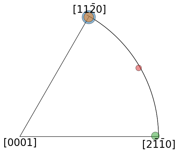
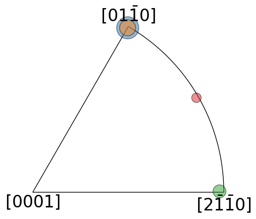
Inspect misorientation axes of clusters in an inverse pole figure
[20]:
cluster_sizes = all_cluster_sizes[1:]
cluster_sizes_scaled = 1000 * cluster_sizes / cluster_sizes.max()

fig = plt.figure(figsize=(6, 6))
ax = fig.add_subplot(projection="ipf", symmetry=sym)
ax.scatter(
    cluster_means.axis, c=colors, s=cluster_sizes_scaled, alpha=0.5, ec="k"
)
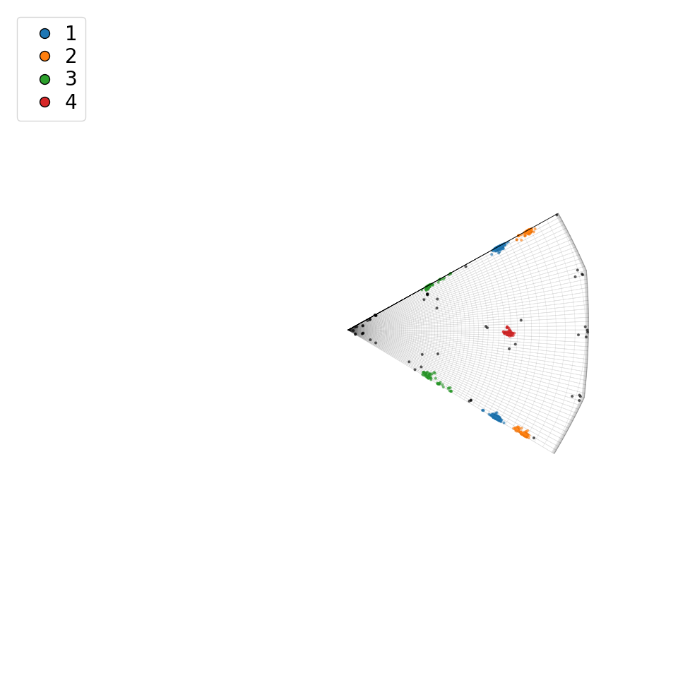
Plot a top view of the misorientation clusters within the fundamental zone for the (D6, D6) bicrystal symmetry
[21]:
wireframe_kwargs = dict(
    color="black", linewidth=0.5, alpha=0.1, rcount=361, ccount=361
)
fig = mori.scatter(
    projection="axangle",
    wireframe_kwargs=wireframe_kwargs,
    c=labels_rgb.reshape(-1, 3),
    s=4,
    alpha=0.5,
    return_figure=True,
)
ax = fig.axes[0]
ax.view_init(elev=90, azim=-60)

handle_kwds = dict(marker="o", color="none", markersize=10)
handles = []
for i in range(n_clusters):
    line = Line2D(
        [0], [0], label=i + 1, markerfacecolor=colors[i], **handle_kwds
    )
    handles.append(line)
ax.legend(
    handles=handles,
    loc="upper left",
    numpoints=1,
    labelspacing=0.15,
    columnspacing=0.15,
    handletextpad=0.05,
);
Plot side view of misorientation clusters in the fundamental zone for the (D6, D6) bicrystal symmetry
[22]:
fig2 = mori.scatter(
    return_figure=True,
    wireframe_kwargs=wireframe_kwargs,
    c=labels_rgb.reshape(-1, 3),
    s=4,
)
ax2 = fig2.axes[0]
ax2.view_init(elev=0, azim=-60)
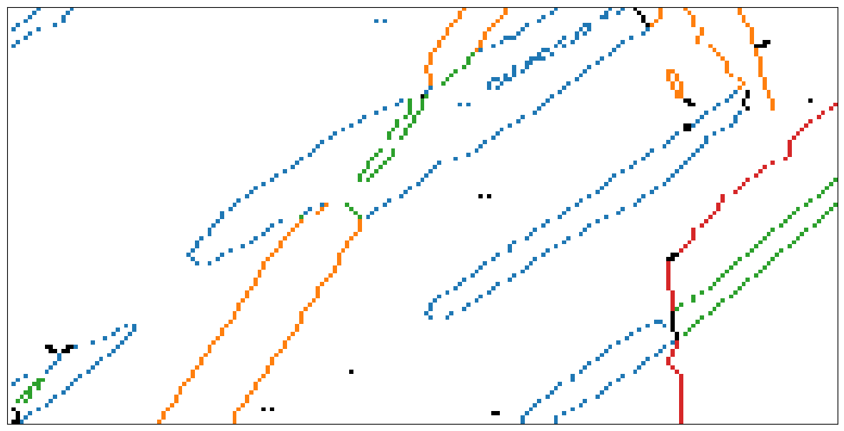
Generate map of boundaries colored according to cluster membership
[23]:
Plot map of boundaries colored according to cluster membership
[24]:
fig3, ax3 = plt.subplots(figsize=(15, 10))
ax3.imshow(mapping)
ax3.set(xticks=[], yticks=[]);